import Pkg
Pkg.activate(@__DIR__)
Pkg.instantiate()HW 1 Solutions
Load Environment
The following code loads the environment and makes sure all needed packages are installed. This should be at the start of most Julia scripts.
Standard Julia practice is to load all needed packages at the top of a file. If you need to load any additional packages in any assignments beyond those which are loaded by default, feel free to add a using statement, though you may need to install the package.
using Random # allows for random seed generation
using Plots # basic plotting: can also install and use other packages
using Graphs # for making graphs and networks
using GraphRecipes # basic graph generation
using LaTeXStrings # allows for LaTeX formatting in plots
using Distributions # sampling and fitting of probability distributions
using CSV # file I/O for CSV files
using DataFrames # data structure for tabular data
# this sets a random seed, which ensures reproducibility of random number generation. You should always set a seed when working with random numbers.
Random.seed!(1)TaskLocalRNG()Problems (Total: 50 Points)
Problem 1 (10)
Problem 1.1 (2)
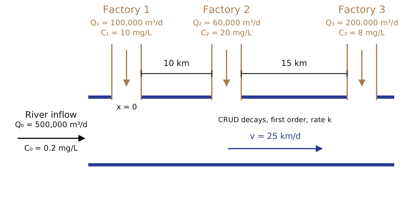
An example diagram might look like this:
Problem 1.2 (5)
The first observation is that between factory, the highest concentration is at the earlier factory’s discharge, as CRUD only decays as it flows downriver and there are no intermediate sources. Thus if the river is in compliance at every discharge, it will be in compliance everywhere else. As a result, we only need to calculate conditions for compliance at the three river discharges.
Factory 1: The inflow mass of CRUD is \[\frac{0.2 \text{mg}}{\text{L}} \times \frac{1 \text{L}}{1000 \text{mg}} \times \frac{500,000 \text{L}}{\text{d}} = 100 \text{mg}.\]
The pre-treatment effluent mass from Factory 1 is (similarly) \(1000 \text{mg}\), so with a treatment level of \(E_1\) Factory 1 would release \(1000 (1 - E_1) \text{mg}\), for a combined mass of \(1100 - 1000 E_1 \text{mg}\). Since the total volume of combined water (inflow + effluent) is \(600 \text{L}\), the comparison of the concentration to the regulatory requirement is \[ \begin{aligned} C_1 = \frac{1100 - 1000E_1}{600} &\leq 1 \text{mg/L} \\ 1000 E_1 &\geq 500 \\ E_1 &\geq 0.5. \end{aligned} \]
Factory 2: To find the inflow mass, we need to look at the decay of the CRUD downstream from the Factory 1 release. Since the first-order decay rate is \(k=0.45 \text{d}^{-1}\), the differential equation for CRUD’s mass is \(M'(t) = -0.45dt\), and the solution is \[M(t) = M_0\exp(-0.45t).\] We want to rewrite this in terms of distance, rather than time, which we can do using the river’s velocity, \(25 \text{km/d}\). This means that in time $t , the river travels \(x = 25 t \text{km}\), so \(t = x / 25\) and the differential equation is \[M(x) = M(0)\exp(-0.45x / 25).\] The initial condition is the mass from the Factory 1 release, which from before is \[M(0) = 1100 - 1000E_1 \text{mg},\] so after \(x = 10 \text{km}\), the mass is \[M(10) = (1100 - 1000E_1)\exp(-0.18) \text{mg}.\] With treatment level \(E_2\), Factory 2 releases \(1200(1-E_2) \text{mg}\), and the combined volume is \(660 \text{L}\), so the concentration condition is \[ \begin{aligned} C_2 = \frac{(1100 - 1000E_1)\exp(-0.18) + 1200(1-E_2)}{660} &\leq 1 \text{mg/L} \\ 2119 - 835 E_1 - 1200 E_2 &\leq 660 \\ 835E_1 + 1200 E_2 &\geq 1459. \end{aligned} \]
Factory 3: This follows an analogous calculation as above, with the new inflow initial condition the mass from the Factory 1 release and the distance downstream \(x=15 \text{km}\). The concentration condition becomes \[ \begin{aligned} 3217 - 637E_1 - 916E_2 - 1600E_3 &\leq 860 \\ 637E_1 + 916 E_2 + 1600 E_3 &\geq 2357. \end{aligned} \]
So to summarize, the three conditions for compliance are: \[ \begin{aligned} E_1 &\geq 0.5 \\ 835E_1 + 1200 E_2 &\geq 1459 \\ 637E_1 + 916 E_2 + 1600 E_3 &\geq 2357. \end{aligned} \]
Problem 1.3
There is no “right” answer to this question, it’s more about reasoning through some relevant considerations. For example:
The total cost for treatment levels \(E_1\), \(E_2\), and \(E_3\) is \[Z = 50 (100)E_1^2 + 50 (60)E_2^2 + 50(200)E_3^2 = 5000E_1^2 + 3000E_2^2 + 10000E_3^2.\] So it is most cost effective for Factory 2 to maximize its treatment. On the other hand, this is also because Factory 2 emits the least effluent, though it is the most concentrated. But the total mass is less than that released by Factory 3. Factory 1 emits a moderate amount of effluent and it is only slightly more concentrated than Factory 3’s. So we might say that Factory 1 should do its minimum level or close to it, then rely on Factory 2 and Factory 3 to do their part to ensure compliance downriver, and asking Factory 2 or Factory 3 to do more might depend on whether want to penalize the concentration of effluent or the mass emitted.
All this is to say: it would be nice to have a more principled approach to making these decisions! We will see one approach to this when we discuss optimization, though we could also use simulation to explore the tradeoffs between cost and concentrations as we vary the three treatment levels systematically.
Problem 2 (6)
The change to the rate constant means that the new constant is \(\alpha' = 0.9 \alpha = 9/200 \text{d}^{-1}\). Let’s denote the new steady-state values by \(X_1'\), \(X_2'\), and \(X_3'\). The other rate constants are still the same: \(\gamma = 1/4 \text{d}^{-1}\) and \(\beta = 10/4 (\text{d}\mu\text{mol}/\text{L})^{-1}\). Since \(\gamma\) and \(\beta\) are the same, the steady-state condition for \(X_1'\) means \(X_2' = \gamma/\beta = 0.1 \mu\text{mol}/\text{L}\), the same as before.
However, now our only independent equation from the steady-state conditions is \[\gamma X_1' = \alpha' X_3'.\] To get another equation, we know that there is no change to the overall mass, so \[X_1' + X_3' = X_1 + X_3 = 1.2 \mu\text{mol}/\text{L}.\] Thus \(X_1' = 1.2 - X_3'\), and substituting (and putting all of the values over a common denominator), \[ \begin{aligned} \frac{60}{200} - \frac{50}{200}X_3' &= \frac{9}{200}X_3' \\ X_3' = \frac{60}{59} \approx 1.02 \mu\text{mol}/\text{L}. \end{aligned} \] Therefore \(X_1' \approx 0.18\). So the net effect of the reduced rate constant is not to change the amount of inorganic P (\(X_2'\)), but to reduce slightly the amount which resides in living organic matter, as the uptake from decomposing matter to living matter requires passing through the inorganic pathway.
Problem 3.1 (3)
The error is that the code initializes the minimum value (min_value) at 0, which is below any of the values in array_values. Instead, if we initialize min_value = array[1], any smaller values will be identified by the loop.
A correct solution might look like:
function minimum(array)
    # initialize the minimum value counter
    min_value = array[1]
    # update minimum values
    for i in 2:length(array)
        if array[i] < min_value
            min_value = array[i]
        end
    end
    # return found minimum
    return min_value
end

array_values = [89, 90, 95, 100, 100, 78, 99, 98, 100, 95]
@show minimum(array_values);
minimum(array_values) = 78Problem 3.2 (3)
The line producing the MethodError is outcomes[i] = (sum(passadieci()) > 11). The problem is actually with a prior line, outcomes = zero(n_trials), which creates outcomes.
zero() is the Julia function to get a zero element (the additive identity) based on the type of the input. For example:
zero(3)0zero(3.0)0.0zero(false)falseSince zero() returns a scalar element (as seen in the examples), trying to index its output with outcomes[i] results in the error, as Julia does not know how to index into a scalar (in this case, an Int).
However, the goal of the relevant line in the script is to initialize a vector consisting of zeros with length n_trials. What we actually want is the function zeros(). Fixing this gets rid of the error (I’ve also fixed another error with the code, namely the threshold for a “win”, but this isn’t essential for this problem):
# function to simulate a passadieci roll: 3 6-sided dice
function passadieci()
    # this rand() call samples 3 values from the vector [1, 6]
    roll = rand(1:6, 3)
    return roll
end
# set number of trials and initialize outcome vector
n_trials = 1_000
outcomes = zeros(n_trials)
# simulate number of passadieci rolls and count wins
for i = 1:n_trials
    outcomes[i] = (sum(passadieci()) >= 11)
end
win_prob = sum(outcomes) / n_trials # compute average number of wins
@show win_prob;
win_prob = 0.502Problem 2.3 (3)
The line that causes the error is return vect - m. The problem is that Julia does not make assumptions about how to handle ambiguous operations like adding or subtracting a scalar (m) from a vector (vect): is this intended and should be done element-wise, or is it a sign that the wrong type was passed (e.g. the other input was intended to be a vector)? To make the intent of the coder explicit, Julia asks that you broadcast an operation that is intended to be applied to a scalar (such as addition or subtraction of another scalar) to be applied element-wise to a vector, instead of assuming that this is the intended behavior.
To broadcast a function f() over a vector v, you use a period, as in f.(v). In this case, we want to change the problematic line to return vect .- m:
# function to remove mean from a vector
function remove_mean(vect)
    # fucntion to compute the mean
    function compute_mean(vect)
        element_sum = 0 # initialize sum
        # compute mean and return
        for v in vect
            element_sum += v
        end
        return element_sum / length(vect)
    end

    m = compute_mean(vect) # compute mean
    # return demeaned vector
    return vect .- m
end

random_vect = rand(1_000)
@show mean(remove_mean(random_vect));
mean(remove_mean(random_vect)) = -1.736388810513745e-16Problem 4 (5)
Problem 4.1 (2)
While we could load the data into a generic array, the most mature data structure for tabular data is in Julia is a DataFrame (from DataFrames.jl, akin to Python’s pandas or R’s dataframes). To load the dataset, we will use CSV.jl’s read() function:
1dat = CSV.read("data/fha.csv", DataFrame)- 1
-
DataFrameis the “sink”, or the datastructure thatCSV.read()will read the file into. There are many options for how to customize theread()function for the specifics of a given CSV file.
ArgumentError: "data/fha.csv" is not a valid file or doesn't exist
Stacktrace:
 [1] CSV.Context(source::CSV.Arg, header::CSV.Arg, normalizenames::CSV.Arg, datarow::CSV.Arg, skipto::CSV.Arg, footerskip::CSV.Arg, transpose::CSV.Arg, comment::CSV.Arg, ignoreemptyrows::CSV.Arg, ignoreemptylines::CSV.Arg, select::CSV.Arg, drop::CSV.Arg, limit::CSV.Arg, buffer_in_memory::CSV.Arg, threaded::CSV.Arg, ntasks::CSV.Arg, tasks::CSV.Arg, rows_to_check::CSV.Arg, lines_to_check::CSV.Arg, missingstrings::CSV.Arg, missingstring::CSV.Arg, delim::CSV.Arg, ignorerepeated::CSV.Arg, quoted::CSV.Arg, quotechar::CSV.Arg, openquotechar::CSV.Arg, closequotechar::CSV.Arg, escapechar::CSV.Arg, dateformat::CSV.Arg, dateformats::CSV.Arg, decimal::CSV.Arg, groupmark::CSV.Arg, truestrings::CSV.Arg, falsestrings::CSV.Arg, stripwhitespace::CSV.Arg, type::CSV.Arg, types::CSV.Arg, typemap::CSV.Arg, pool::CSV.Arg, downcast::CSV.Arg, lazystrings::CSV.Arg, stringtype::CSV.Arg, strict::CSV.Arg, silencewarnings::CSV.Arg, maxwarnings::CSV.Arg, debug::CSV.Arg, parsingdebug::CSV.Arg, validate::CSV.Arg, streaming::CSV.Arg)
   @ CSV ~/.julia/packages/CSV/LiiJM/src/context.jl:314
 [2] #File#32
   @ ~/.julia/packages/CSV/LiiJM/src/file.jl:222 [inlined]
 [3] CSV.File(source::String)
   @ CSV ~/.julia/packages/CSV/LiiJM/src/file.jl:162
 [4] read(source::String, sink::Type; copycols::Bool, kwargs::@Kwargs{})
   @ CSV ~/.julia/packages/CSV/LiiJM/src/CSV.jl:117
 [5] read(source::String, sink::Type)
   @ CSV ~/.julia/packages/CSV/LiiJM/src/CSV.jl:113
 [6] top-level scope
   @ ~/Teaching/BEE4750/fall2026/solutions/hw01/hw01.qmd:245
To find the number of rows and columns of a DataFrame, we can use nrow() and ncol().
@show nrow(dat);
@show ncol(dat);
UndefVarError: `dat` not defined in `Main.Notebook` Suggestion: check for spelling errors or missing imports. Stacktrace: [1] macro expansion @ show.jl:1232 [inlined] [2] top-level scope @ ~/Teaching/BEE4750/fall2026/solutions/hw01/hw01.qmd:252
Problem 4.2 (3)
Calculate the number of miles driven per person per day for every metro area. Make a scatterplot of this on the \(y\)-axis and the population of the city on the \(x\)-axis. Make sure to label your axes and include a caption clearly describing the plot. Highlight where the New York City and Houston metro areas are on the plot and make a legend clearly labelling any plot features.
To see the column names of the data:
names(dat)UndefVarError: `dat` not defined in `Main.Notebook` Suggestion: check for spelling errors or missing imports. Stacktrace: [1] top-level scope @ ~/Teaching/BEE4750/fall2026/solutions/hw01/hw01.qmd:263
So to calculate the number of miles driven per person per day, we would want to divide dat[:, "daily_vmt (mi/day)"] by dat[:, "population"]. We could do this in a few different ways. Either way, we will The first is to use map over eachrows(dat):
1dat[:, "mi_per_pop"] = map(row -> row["daily_vmt (mi/day)"] / row["population"], eachrow(dat))- 1
-
mapapplies a function in the first argument to every “object” in the iterator in the second object. Since we are defining a custom function instead of using one likemeanorsum, we will use an anonymous function specification defined on eachrowand doing the desired division on its elements.eachrow(dat)defines an iterator which processes each row in turn (as though the DataFrame were a vector of rows).
UndefVarError: `dat` not defined in `Main.Notebook`
Suggestion: check for spelling errors or missing imports.
Stacktrace:
 [1] top-level scope
   @ ~/Teaching/BEE4750/fall2026/solutions/hw01/hw01.qmd:269
Similarly, we can broadcast the function over eachrow(dat):
dat[:, "mi_per_pop"] = (row -> row["daily_vmt (mi/day)"] / row["population"]).(eachrow(dat))UndefVarError: `dat` not defined in `Main.Notebook` Suggestion: check for spelling errors or missing imports. Stacktrace: [1] top-level scope @ ~/Teaching/BEE4750/fall2026/solutions/hw01/hw01.qmd:275
To make the scatterplot, we can use Plots.scatter() (though you could install and use one of the other Julia plotting packages as well):
- 1
-
The
labelkeyword assigns a name to the entry in the legend corresponding to what is being plotted in thescatter()function (similarly for a line plotted byPlots.plot()). - 2
-
xlabel!()andylabel!()are examples of mutating functions, which means they transform the object they’re called on in-place rather than needing to be assigned a new variable. In these cases, the plot object (phere) is optional if you only want to apply it to the last plot you made, but there’s never a downside to making it explicit.
UndefVarError: `dat` not defined in `Main.Notebook`
Suggestion: check for spelling errors or missing imports.
Stacktrace:
 [1] top-level scope
   @ ~/Teaching/BEE4750/fall2026/solutions/hw01/hw01.qmd:280
We can add the NYC and Houston points by plotting them specifically with a different color and a specific legend option (we’ll also add the caption here). By inspecting the data, we can see that the NY metro area is the first row, while Houston is the 7th.
1scatter!(p, dat[[1], "population"], dat[[1], "mi_per_pop"], color="red", label="New York")
scatter!(p, dat[[7], "population"], dat[[7], "mi_per_pop"], color="orange", label="Houston")- 1
-
A quirk of
Plots.jlis that scatterplots have to be for entire vectors, not individual points, so an individual point needs to be wrapped as a 1-element vector.
UndefVarError: `dat` not defined in `Main.Notebook`
Suggestion: check for spelling errors or missing imports.
Stacktrace:
 [1] top-level scope
   @ ~/Teaching/BEE4750/fall2026/solutions/hw01/hw01.qmd:293
Problem 5 (20)
Problem 5.1
A = [0 1 1 1;
    0 0 0 1;
    0 0 0 1;
    0 0 0 0]

nodes = ["Plant", "Land Treatment", "Chem Treatment", "Pristine Brook"]
# modify this dictionary to add labels
edge_labels = Dict((1, 2) => L"$X_1$", (1,3) => L"$X_2$", (1, 4) => L"$X_3$",(2, 4) => L"$0.2X_1$",(3, 4) => L"$0.005X_2^2$")
shapes=[:hexagon, :rect, :rect, :hexagon]
xpos = [0, -1.5, -0.25, 1]
ypos = [1, 0, 0, -1]

p = graphplot(A, names=nodes, edgelabel=edge_labels, markersize=0.15, markershapes=shapes, markercolor=:white, x=xpos, y=ypos)
display(p)Problem 5.2 (4)
These equations will be derived in terms of \(X_1\) (the land disposal amount, in kg/day) and \(X_2\) (the chemically treated amount, in kg/day), where \(X_1 + X_2 \leq 100\ \mathrm{kg/day}\). Note that we don’t need to explicitly represent the amount of directly disposed YUK, as this is \(X_3 = 100 - X_1 - X_2\) and so is not a free variable.
The amount of YUK which will be discharged is
\[ \begin{aligned} D(X_1, X_2) &= 100 - X_1 - X_2 + 0.2 X_1 + 0.005X_2^2 \\ &= 100 - 0.8 X_1 + (0.005X_2 - 1)X_2 \\ &= 100 - 0.8 X_1 + 0.005 X_2^2 - X_2 \end{aligned} \]
The cost is \[ C(X_1, X_2) = X_1^2/20 + 1.5 X_2. \]
Problem 5.3 (3)
Implement your systems model as a Julia function which computes the resulting YUK discharge and cost for a particular treatment plan.
Solution:
A Julia function for this model could look like:
# we will assume that X₁, X₂ are vectors so we can vectorize
# the function; hence the use of broadcasting. This makes unpacking
# the different outputs easier as each will be returned as a vector.
# Note that even though this is vectorized, passing scalar inputs
# will still work fine.
function yuk_discharge(X₁, X₂)
    # Make sure X₁ + X₂ <= 100! Throw an error if not.
1    if any(X₁ .+ X₂ .> 100)
        error("X₁ + X₂ must be less than 200")
    end
2    yuk = 100 .- 0.8X₁ .+ (0.005X₂ .- 1) .* X₂
    cost = X₁.^2/20 .+ 1.5X₂
    return (yuk, cost)
end- 1
- Checking for these kinds of errors is useful when there are hard limits on what arguments can be passed in. This syntax lets you throw an error which says something is going wrong in the code. In general, Julia style is to try to do a computation and throw an error if something goes wrong.
- 2
- We use broadcasting here to work on vectors of arguments for efficiency. This is in no way required.
yuk_discharge (generic function with 1 method)I will use a \(\text{Dirichlet}(3, 1)\) distribution to draw 1,000 3-d vectors adding up to 1 for testing, but you could also loop over a grid of values for \(X_1\) and \(X_2\) (since \(X_3\) is determined by those two) and evaluate.
- 1
-
rand(D, n)draws n samples from aDistributionobjectD. We will see this again later when we talk about simulation and Monte Carlo. Also, since the Dirichlet distribution samples values between 0 and 1, I have to multiply by 100 to scale to wastewater volumes due to how I designedyuk_discharge. - 2
-
a, b = ...unpacks a tuple(a, b)into variablesaandbwithout needing to explicitly use an intermediate step, e.g.tup = ...,a = tup[1],b = tup[2], which we could also have done. This is why I set upyuk_dischargeto return a tuple, though there are other options. For example,yuk_dischargecould have returned a vector, and a comprehension could have unpacked that into the two components, or you could have used two different functions for cost and concentration. This is why we aren’t grading your code: there are many roads which lead to Rome!
([82.64022699576161, 31.681515467607312, 53.97979142744385, 38.09941279111079, 34.75224900866194, 85.84911471487678, 38.019552492009, 43.28367061001507, 74.88978068034905, 55.6278579476064 … 23.992732714301304, 51.23508924178167, 73.27511020738929, 25.34609784891812, 41.40711743286863, 46.514686003206315, 77.62677443874955, 58.15508592022454, 77.94343946832551, 41.447902332877], [19.33668253359526, 158.22965370685597, 142.48667238668858, 131.24095400324697, 288.1570103910447, 15.058362100355158, 134.2522596125352, 107.28139653342407, 34.123598879715544, 94.80414114093286 … 187.92350896851224, 97.64800307824338, 37.493226660033066, 408.0457037167852, 118.35498313303957, 128.4873779266283, 28.427265852989926, 77.72954336302251, 28.286350124521398, 135.6347203586801])Now let’s plot the results, using scatter().
p = scatter(D, C, markersize=2, label="Treatment Samples")
# Label axes
xaxis!(p, "YUK Discharge (kg/day)")
# For the y-axis label, we need to "escape" the $ by adding a slash
# otherwise it interprets that as starting math mode
yaxis!(p, "Treatment Cost (\$/day)")Problem 5.4 (3)
1vline!(p, [20], color=:red, label="Regulatory Limit")- 1
-
This is how to add a vertical line to a plot with a label. The syntax for a horizontal line is
hline(...).
We can see that there are a few treatment strategies which comply with the limit, namely:
1is_compliant = D .< 20
sum(is_compliant)- 1
-
D .< 20creates a Boolean vector based on the condition, thensumgives us the number of elements which passes the condition.
14However, they are fairly expensive. The minimum cost of these strategies is
minimum(C[is_compliant])248.20228150293696Problem 5.5 (4)
While there is a tradeoff between cost and the discharge, there are some strategies which cost the same as compliant strategies and don’t achieve compliance with the standard. As a result, while you need to spend a certain amount of money, that doesn’t guarantee compliance — how that money is allocated across the strategies matters as well.
Problem 5.6 (4)
To minimize these functions, we want to look at either the critical points (where the partial derivatives are zero) or at the constraints. For cost, \(dC/dX_2 = 1.5\) is never zero, so there are no critical points. However, the lowest-cost point occurs at the boundary \(X_2 = 0\) and \(X_1 = 0\), where there is no cost (unsurprisingly, doing nothing often costs the least). But this does not comply with the constraint, as the YUK discharge is 100 kg/day.
The YUK discharge function \(D\) has the following partial derivatives:
\[ \begin{aligned} \frac{\partial D}{\partial X_1} &= -0.8 \\ \frac{\partial D}{\partial X_2} &= 0.01 X_2 - 1, \end{aligned} \]
so we need to check the values along the boundaries \(X_1 = 100 - X_2\), \(X_1 = 0\), and \(X_2 = 0\). \[D(100 - X_2, X_2) = 20X_2 - 0.005 X_2^2,\] which has a partial derivative \[\frac{\partial D}{\partial X_2}(100 - X_2, X_2) = -0.2 + 0.01 X_2.\] This has a minimum at \(X_2 = 20\) and therefore \(X_1 = 80\), with a corresponding YUK discharge of 18 kg/day. If \(X_2 = 0\), the minimum value (at \(X_1 = 100\)) is a discharge of 20 kg/day, while the minimum value along \(X_1 = 0\) is 50 kg/day (\(X_2 = 100\)). Thus, the minimum occurs at \(X_1 = 80\) and \(X_2 = 20\), with a corresponding cost of $350/day.
Adding these points to the plot:
# least cost solution
least_cost = yuk_discharge(0, 0)
scatter!(p, least_cost, color=:orange, label="Least Cost Solution")
# least discharge solution
least_discharge = yuk_discharge(80, 20)
scatter!(p, least_discharge, color=:purple, label="Least Discharge Solution")The least-cost solution, unsurprisingly, would be pretty bad given how much the YUK discharge violates the regulatory constraint. However, the least-discharge solution looks pretty good: there are more expensive treatment plans which comply with the regulatory constraint, but not many that are less expensive.
References
List any external references consulted, including classmates.