Gaussian Plumes: Deriving the Model

---

Lecture 10

September 30, 2026

Overview

• Review of Last Class
• The Gaussian Plume Model
• Dispersion and Atmospheric Stability
• Key Takeaways
• Upcoming Schedule
• Appendix
• References

Review of Last Class

Monte Carlo vs. Discretization Error

Discretization

• pick \(\Delta t\) from a characteristic timescale
• halve it; see if the answer moves
• error scales linearly with \(\Delta t\)

Monte Carlo

• pick \(n\) from a target CI half-width
• double it; see if the estimate moves
• error scales as \(\sim 1/\sqrt{n}\)

Questions?

Text: VSRIKRISH to 22333

URL: https://pollev.com/vsrikrish

See Results

The Gaussian Plume Model

Some Approaches for Modeling Air Pollution

So far: box (airshed) models — overall mass balance across a whole region.

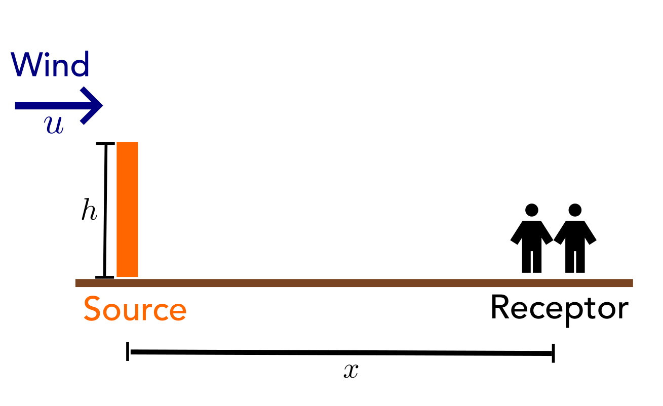
Today: point sources and receptors — plume models, which track concentration as a continuous function of position relative to a source.

Point Sources and Receptors

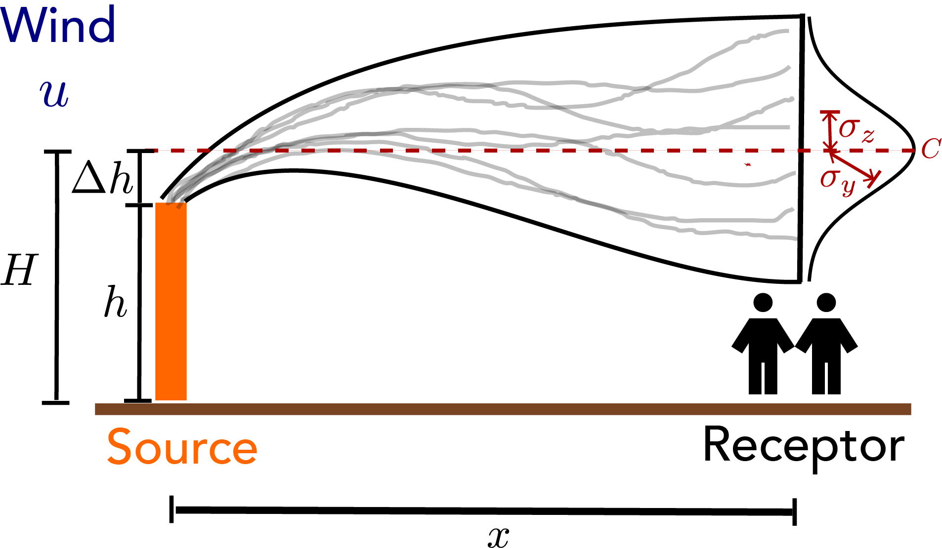
Point Source/Receptor Schematic

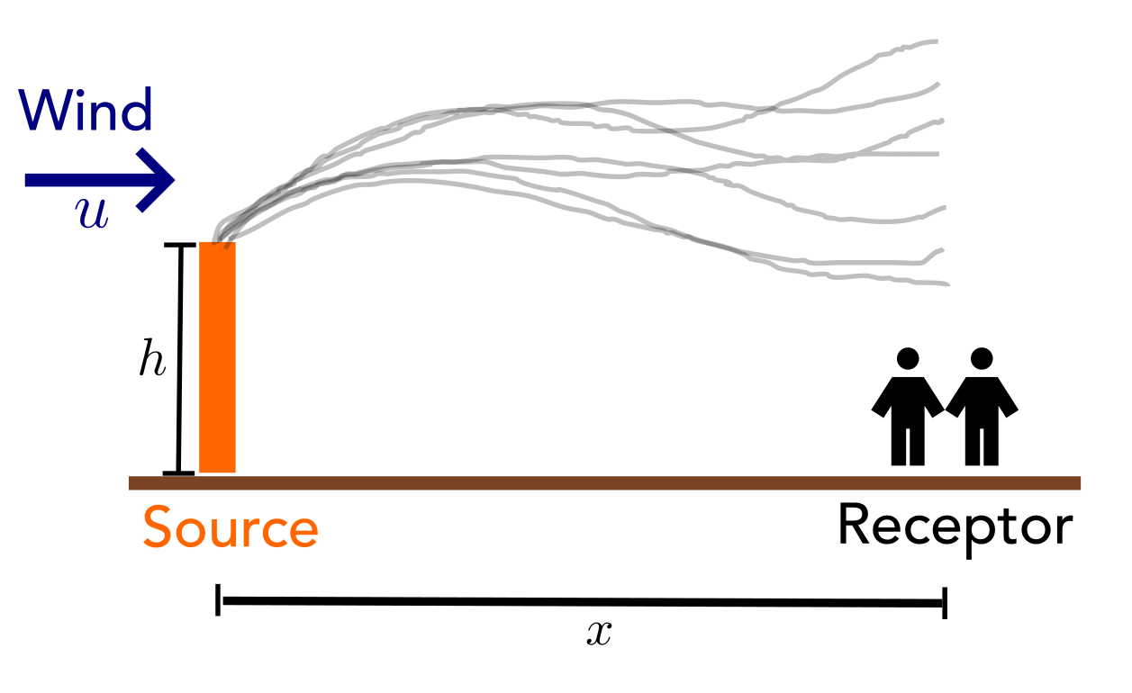
Individual Paths of Emissions

Point Source Flow Traces

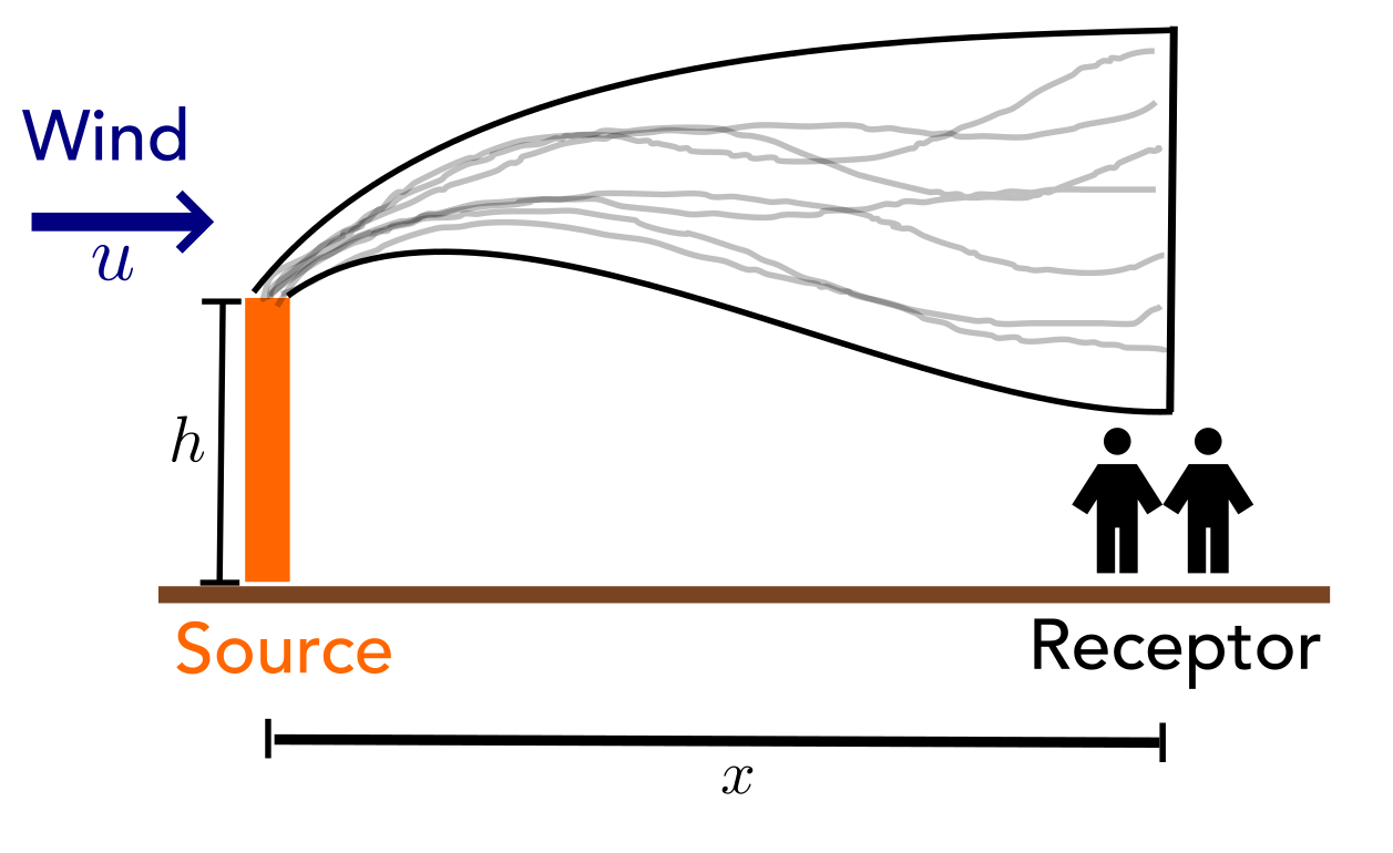
Plume: Time-Averaged Positions

Point Source Average Plume

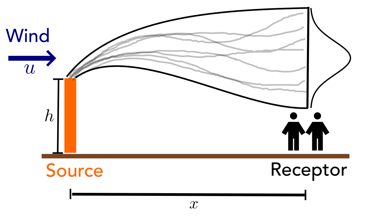
“Gaussian Plume”

Gaussian Plume

“Gaussian Plume”

Gaussian Plume Distribution

The Advection-Diffusion Equation

The mass balance of a small air control volume:

\[\frac{\partial C}{\partial t} = \underbrace{\sum_{i=x,y,z}(D+K_{ii})\frac{\partial^2 C}{\partial x_i^2}}_{\text{diffusion}} - \underbrace{\vec{u}\cdot\vec{\nabla}C}_{\text{advection}} + \underbrace{S}_{\text{reactions}}\]

\(D\): molecular diffusion; \(K_{ii}\): turbulent mixing in direction \(i\); \(S\): reactions (none here).

Full derivation, step by step: appendix.

This is the same mass balance as the box and DO models, applied to a tiny cube of air instead of a whole airshed or river reach. Pollutant in the cube changes because the wind carries it in or out (advection), because it spreads from crowded places to less crowded ones (diffusion, molecular and turbulent), or because it reacts. Everything that follows is deciding which of these terms we can ignore for a smokestack plume. The appendix has every step with the math.

Diffusive Flux

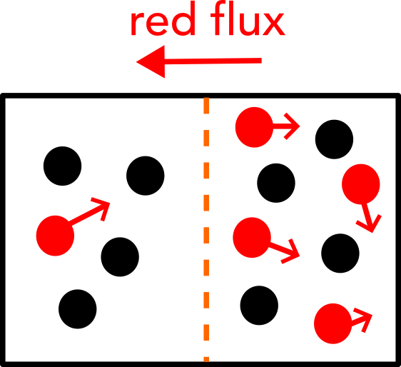
Diffusive Flux

Concentration gradient + diffusion \(\Rightarrow\) flux.

Fick’s law: \[F_x = -D\frac{dC}{dx}\]

Fick’s law comes from random molecular motion. Molecules jiggle in every direction, and wherever there are more of them, more wander out than wander in. The net result is a flow from high to low concentration, proportional to how steep the difference is, which is why there is a minus sign. Fick found it in 1855 by analogy with Fourier’s law for heat. D is a property of the gases themselves, and it is tiny: about a hundred-thousandth of a square metre per second for a gas in air.

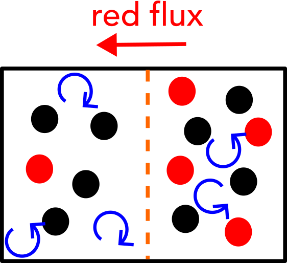
Where Turbulent Flux Comes From

The plume is the time average of the individual puffs. Split wind and concentration into mean and fluctuation, \(u = \bar u + u'\) and \(C = \bar C + c'\). Averaging the advective flux leaves an extra term:

\[\overline{uC} = \bar u\,\bar C + \overline{u'c'}\]

\(\overline{u'c'}\) is pollutant carried by eddies. K-theory closes it by analogy with Fick’s law: \(\overline{u'c'} = -K_{xx}\,\partial \bar C/\partial x\).

We are not predicting where the smoke is at one instant; that is the wiggly puffs in the earlier figure. We are predicting the average concentration over roughly an hour. When you average the wind carrying the pollutant, most of the cross terms average to zero, but one survives: the correlation between gusts and concentration. Below the plume centreline, for example, updrafts bring up cleaner air and downdrafts bring down dirtier air, so on average pollutant moves downward, from high to low concentration, just like diffusion. K-theory says to treat this like Fick’s law, with eddies playing the role of molecules.

Turbulent Flux

Turbulent Flux

Concentration gradient + turbulent mixing \(\Rightarrow\) flux.

\[F_x = -K_{xx}\frac{dC}{dx}\]

\(K_{xx}\) depends on flow/eddy characteristics.

Same form as Fick’s law, but K describes the eddies, not the air. A rough way to think about it: K is an eddy’s speed times the distance it carries a parcel before mixing in. That is about half a metre per second times tens of metres, so tens of square metres per second. Molecules follow the same recipe with a tiny step, which is why D is about a million times smaller. K also differs by direction: vertical mixing is suppressed when the atmosphere is stable, which is where stability classes come in later.

Assumption 1: Steady State

\[\cancel{\frac{\partial C}{\partial t}} = \sum_{i=x,y,z}(D+K_{ii})\frac{\partial^2 C}{\partial x_i^2} - \vec{u}\cdot\vec{\nabla}C\]

Constant emissions and weather over the averaging period.

Steady state means we describe the plume averaged over a period when the stack emits at a constant rate and the weather holds steady, typically about an hour. It does not mean nothing moves; the air is moving the whole time. It means the averaged picture is not changing. If emissions or the wind shift during the hour, the model describes a blend of conditions, and the real footprint wanders around.

Assumption 2: Wind Only Along \(x\)

\[\vec{u}\cdot\vec\nabla C = u_x\frac{\partial C}{\partial x} + \cancel{u_y\frac{\partial C}{\partial y}} + \cancel{u_z\frac{\partial C}{\partial z}}\]

Part of this is just a choice: we point the x axis along the average wind, so by definition there is no mean wind across it. The real assumption is that the wind is uniform, with the same speed and direction everywhere, including at every height. Real wind speeds up with height, and that is one of the first things more advanced models relax. This is only about the mean wind; the gusts are still there, hiding inside K.

Assumption 3: Turbulence Dominates Molecular Diffusion

\(D \sim 10^{-5}\) m²/s for a gas in air; \(K \sim 1\)–\(100\) m²/s. Five or more orders of magnitude apart:

\[(\cancel{D}+K_{ii})\frac{\partial^2 C}{\partial x_i^2} \approx K_{ii}\frac{\partial^2 C}{\partial x_i^2}\]

This one is just a size comparison. In the atmosphere, molecular diffusion is roughly a million times weaker than turbulent mixing, so dropping it changes nothing you could measure. It is the same reason stirring coffee mixes the milk in seconds, while waiting for diffusion alone would take hours.

Assumption 4: Negligible Along-Wind Dispersion

\(\Delta C\) is how much \(C\) changes over a distance \(L\):

\[\frac{u\,\partial C/\partial x}{K_{xx}\,\partial^2 C/\partial x^2} \sim \frac{u\,\Delta C/L}{K_{xx}\,\Delta C/L^2} = \frac{uL}{K_{xx}} = Pe\]

A Péclet number argument: \(Pe \gg 1\) at meaningful distances downwind, so drop \(K_{xx}\). The crosswind terms stay: mixing is the only transport in \(y\) and \(z\).

Compare how fast the wind carries pollutant downwind with how fast turbulence spreads it along the wind. The wind covers a kilometre in a few minutes; along-wind mixing would take hours to spread pollutant over the same distance. That ratio is the Péclet number, and at a kilometre it is around 50, so along-wind spreading is a correction of a few percent. The estimate only needs rough sizes: the slope is about the change in concentration divided by the distance, and the curvature is that slope divided by the distance again. The size of the change cancels in the ratio, so only the distance matters. Why not drop the crosswind terms the same way? Because there is no wind across the plume to compete with: mixing is the only thing moving pollutant sideways. The plume is also narrow, so concentration changes sharply across it, which makes the crosswind terms as large as the advection term. They are what balance it.

Péclet Number Downwind

u_wind, Kxx = 2.5, 50
Lvals = 100:50:10000
Pe = u_wind .* Lvals ./ Kxx
plot(Lvals ./ 1000, Pe, xlabel="Distance  [km]", ylabel=L"Pe = uL/K_{xx}",
    color=cb_vermillion, linewidth=4, legend=false, yscale=:log10)
hline!([1], color=:black, linestyle=:dash, linewidth=2)
plot!(size=(950, 400), left_margin=12mm, right_margin=8mm,
    bottom_margin=12mm, top_margin=5mm)

Figure 1: Péclet number for along-wind transport, u = 2.5 m/s, Kxx = 50 m²/s.

Pe grows linearly with distance. With these numbers it passes 1 at about 20 metres and 10 at about 200 metres, so beyond a few hundred metres along-wind dispersion really is negligible. The assumption fails right next to the stack, which is also where the plume formula blows up, and in very light winds, where u is small. That is one reason Gaussian plume models are not used in calm conditions.

What’s Left

With these four assumptions:

\[\bbox[5pt, border: 3px solid red]{u\frac{\partial C}{\partial x} = K_{yy}\frac{\partial^2 C}{\partial y^2} + K_{zz}\frac{\partial^2 C}{\partial z^2}}\]

Read this equation as a balance between two things: the wind carrying pollutant downwind on the left, and turbulence spreading it sideways and vertically on the right. There is no time derivative, no along-wind spreading, and no molecular diffusion left. The next move is to see that this is a diffusion equation in disguise.

Boundary Condition

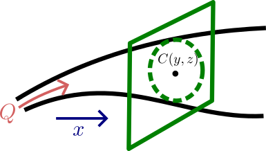
Plus a boundary condition: mass flowing through any downwind cross-section must equal the emission rate \(Q\):

\[Q = \iint u\,C\,dy\,dz\]

Boundary Condition for the A-D Equation

The stack is where the pollutant comes from, and this says none of it disappears. Take any slice across the plume downwind: the wind pushes pollutant through it at some rate, and with steady state and no reactions that rate must equal what the stack emits. Another way to see it: in one second the stack emits Q, and the wind stretches that over u metres of plume, so every metre of plume carries Q divided by u. This is what fixes the overall size of the concentration.

Distance Becomes Travel Time

Let \(\tau = x/u\), the time the air takes to reach \(x\). Then \(u\,\partial C/\partial x = \partial C/\partial \tau\):

\[\frac{\partial C}{\partial \tau} = K_{yy}\frac{\partial^2 C}{\partial y^2} + K_{zz}\frac{\partial^2 C}{\partial z^2}\]

This is the 2-D diffusion (heat) equation: each downwind slice is a puff that has been spreading for time \(x/u\). Its point-source solution is a Gaussian.

This is the key trick. Imagine riding downwind on a thin slice of air, moving at the wind speed. From your seat there is no wind, since you are moving with it; all you see is the pollutant in your slice spreading sideways and up and down. Distance downwind is just how long your slice has been travelling. So the steady plume is a procession of puffs, each a little older than the one behind it. That turns a steady three-dimensional problem into a two-dimensional spreading problem in time, which is the ordinary diffusion equation. It only works because the wind is uniform and because we dropped along-wind spreading; otherwise neighbouring slices would leak into each other.

Solving the PDE

\[C(x,y,z) = \frac{Q}{4\pi x\sqrt{K_{yy}K_{zz}}}\exp\left[-\frac{u}{4x}\left(\frac{y^2}{K_{yy}} + \frac{(z-H)^2}{K_{zz}}\right)\right]\]

Substitute \(\sigma_y^2 = 2K_{yy}\dfrac{x}{u}\), \(\sigma_z^2 = 2K_{zz}\dfrac{x}{u}\) — the distance a diffusing parcel has spread by the time it reaches \(x\).

The diffusion equation starting from a single point has a well-known solution: a bell curve that gets wider and flatter over time while keeping the same total mass. One way to see why: each bit of pollutant has been kicked around by many random eddies, and the sum of many small random kicks is normally distributed, by the central limit theorem. The width grows like the square root of the travel time, the same result as a random walk. Crosswind and vertical spreading happen independently, so the answer is a bell curve across the wind times a bell curve in the vertical. The formula blows up at the stack itself; it describes the plume away from the source.

The Gaussian Plume

\[C(x,y,z) = \frac{Q}{2\pi u\sigma_y\sigma_z}\exp\left[-\frac{1}{2}\left(\frac{y^2}{\sigma_y^2} + \frac{(z-H)^2}{\sigma_z^2}\right)\right]\]

A Gaussian distribution in \(y\) and in \(z\) — which is where the name of the model comes from, and why we use the \(\sigma_y,\sigma_z\) notation.

Rewriting with sigma makes the shape readable: it is two normal distributions, and sigma y and sigma z are their standard deviations, literally how spread out the plume is at that distance. The factor in front is exactly what makes every cross-section carry the full emission rate Q. In theory sigma grows like the square root of distance, but in practice we do not know K well, so we read sigma off empirical curves for each stability class, which comes shortly.

Reflection

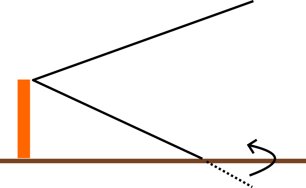
Reflected Mass Off Ground

Pollutant doesn’t vanish into the ground: \(\partial C/\partial z = 0\) at \(z=0\) — a Neumann condition.

Without the ground, the Gaussian from the last slide would let pollutant keep spreading downward, into the earth. For most gases the ground absorbs very little, so pollutant that reaches the surface has nowhere to go but back up. No net flow through the ground means the vertical concentration profile has to arrive at the surface flat, with zero slope. That is a Neumann condition, because it fixes the slope rather than the value. Physically, this is why ground-level concentrations are higher than the no-ground formula predicts: pollutant piles up against the surface instead of passing through it.

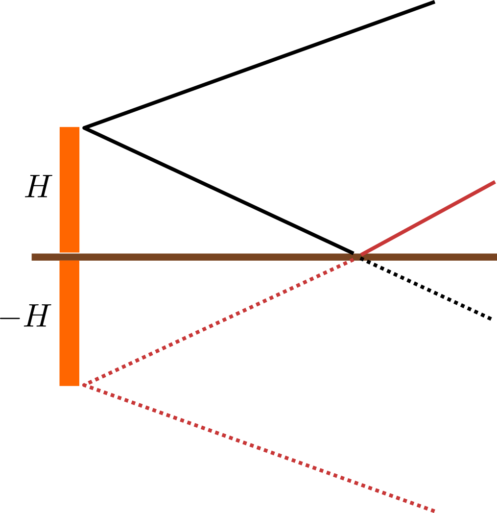
Enforcing It With an Image Source

Add a second, “reflected” source below ground, the mirror image of the real one.

Reflected Mass Off Ground

Think of the ground as a mirror. Put an imaginary second stack the same distance below ground as the real one is above it, emitting the same amount. At the ground the two plumes are exactly symmetric: whatever the real plume would push down through the surface, the imaginary one pushes up by the same amount, so nothing crosses. Above ground, the imaginary plume’s contribution is exactly the pollutant that bounced off the surface. This works because the equation is linear, so solutions can simply be added, and because a mirror-image setup automatically has zero slope at the ground. It is the same method of images used for heat conduction next to an insulated wall. For a ground that absorbed everything, you would give the image the opposite sign instead.

Final Model: Elevated Source With Reflection

\[\begin{aligned} C(x,y,z) &= \frac{Q}{2\pi u\sigma_y\sigma_z}\exp\left(\frac{-y^2}{2\sigma_y^2}\right) \times \\ &\left[\exp\left(\frac{-(z-H)^2}{2\sigma_z^2}\right) + \exp\left(\frac{-(z+H)^2}{2\sigma_z^2}\right)\right] \end{aligned}\]

This is the plume you will actually use: the crosswind bell curve, times a vertical profile made of the real plume plus its mirror image. Two things to point out. At ground level the two vertical terms are equal, so the ground-level concentration is exactly twice what the no-ground formula gives. And the stack height only enters through those two terms: a taller stack pushes both bells further from the ground, which lowers concentrations near the stack and pushes the touchdown point further downwind. In practice H is the effective stack height, the physical stack plus how far the hot, fast exhaust rises before levelling off.

Impact of the Image Term

plume_params = let
    Q, H, u_wind = 100.0, 41.0, 2.5
    (; Q, H, u_wind)
end

sig_y(xk) = 34.0 * xk^0.894
function sig_z(xk)
    if xk < 1
        return 14.35 * xk^0.740 - 0.35
    else
        return 62.6 * xk^0.180 - 48.6
    end
end

function plume(xk, y, z, params; reflect=true)
    sy, sz = sig_y(xk), sig_z(xk)
    base = (params.Q / (2π * params.u_wind * sy * sz)) * exp(-y^2 / (2sy^2))
    real_source = exp(-(z - params.H)^2 / (2sz^2))
    if reflect
        image_source = exp(-(z + params.H)^2 / (2sz^2))
    else
        image_source = 0.0
    end
    return base * (real_source + image_source)
end

dz = 0.001
flux_with = (plume(3.0, 0.0, dz, plume_params) - plume(3.0, 0.0, 0.0, plume_params)) / dz
flux_without = (plume(3.0, 0.0, dz, plume_params; reflect=false) - plume(3.0, 0.0, 0.0, plume_params; reflect=false)) / dz

\(\partial C/\partial z\) at the ground, 3 km downwind: with the image term, 1.3e-9; without it, 4.5e-5 — about \(3\times 10^4\) times larger.

This checks the boundary condition numerically. We estimate the vertical slope of the concentration right at the ground, 3 km downwind, with a tiny finite difference. With the image term the slope is essentially zero, so nothing leaks through the ground. Without it, the slope is tens of thousands of times larger, meaning pollutant is flowing down into the earth. The second exponential is not decoration; it is the boundary condition. Note what this does and does not show: it confirms we solved the equation we wrote down, not that the equation describes real terrain.

Final Model Assumptions

1. Steady-state
2. Constant wind velocity and direction
3. Turbulent mixing \(\gg\) molecular diffusion
4. Wind \(\gg\) dispersion in the \(x\)-direction
5. No reactions
6. Smooth ground (no extra turbulent eddies or reflections)

Each item comes from a specific step. Steady state and a uniform wind removed the time derivative and the crosswind wind; the size comparison removed molecular diffusion; the Péclet argument removed along-wind dispersion; no reactions removed the source term; and a flat ground that neither absorbs nor adds turbulence gave us the image source. Each is also a place the model can fail: winds that shift during the hour, near-calm conditions, receptors very close to the stack, pollutants that react or deposit over long distances, and hills or buildings. When you use the model, ask which of these your situation strains most. That question is where model validation picks up.

Dispersion and Atmospheric Stability

Estimating Dispersion “Spread”

\(\sigma_y,\sigma_z\) matter enormously for the plume’s footprint. What sets them?

Main driver: atmospheric stability — greater stability means less vertical/cross-wind spreading.

Pasquill (1961): six stability classes.

Atmospheric Stability Classes

Class	Stability	Description
A	Extremely unstable	Sunny summer day
B	Moderately unstable	Sunny & warm
C	Slightly unstable	Partly cloudy day
D	Neutral	Cloudy day or night
E	Slightly stable	Partly cloudy night
F	Moderately stable	Clear night

Source: https://courses.ecampus.oregonstate.edu/ne581/eleven/

Estimating Dispersion “Spread”

\[\sigma_y = ax^{0.894}, \qquad \sigma_z = cx^d + f\]

Dispersion Coefficients

Source: https://courses.washington.edu/cee490/DISPCOEF4WP.htm

Note: here \(x\) is in km, while \(y,z\) in the plume equation are in m.

Example

The emission rate of SO\(_2\) from a smokestack is 100 g/s. At 3 km downwind on a clear fall evening (class F), what is the centerline ground-level concentration of SO\(_2\)? Effective plume height is 41 m; wind speed at that height is 2.5 m/s.

\[\sigma_y = 34x^{0.894} \qquad \sigma_z = \begin{cases}14.35x^{0.740}-0.35 & x<1\text{ km} \\ 62.6x^{0.180}-48.6 & x>1\text{ km}\end{cases}\]

Plugging in The Numbers

xk = 3.0
sy, sz = sig_y(xk), sig_z(xk)
Cground = plume(xk, 0.0, 0.0, plume_params)
println("σ_y = ", round(sy, digits=1), " m")
println("σ_z = ", round(sz, digits=1), " m")
println("C(3 km, 0, 0) = ", round(Cground * 1e6, digits=1), " µg/m³")

σ_y = 90.8 m
σ_z = 27.7 m
C(3 km, 0, 0) = 1692.2 µg/m³

• Centerline, ground level: \(y=0,\ z=0\)
• \(\sigma_y \approx\) 91.0 m, \(\sigma_z \approx\) 28.0 m
• \(C \approx\) 1692.0 µg/m\(^3\)

Key Takeaways

Key Takeaways

• The plume equation is based on the advective-diffusion equation.
• Number of key assumptions: when do they hold and when don’t they?
• \(\sigma_y,\sigma_z\) are empirical, tied to atmospheric stability class — not derived from first principles.

Upcoming Schedule

Next Classes

Monday: Quiz 2, then simulating the plume model

Wednesday: Model calibration and validation.

Assessments

Mini-Project 1: Due Thursday, October 22.

Quiz 2: Monday, October 5, covering discretization, convergence, Streeter-Phelps, and Monte Carlo.

Appendix

Deriving the Plume: Mass Balance

The same bookkeeping as the box and DO models, on a small cube of air \(dx\,dy\,dz\):

\[\frac{\partial C}{\partial t} = -\nabla\cdot\vec F + S\]

• \(\vec F\): flux of pollutant through the cube’s faces [mass/(area·time)]
• \(S\): reactions or sources inside the cube

As the cube shrinks, “outflow minus inflow” per unit volume becomes the divergence \(\nabla\cdot\vec F\).

Contributions to Flux

\[\vec F = \underbrace{\vec u\,C}_{\text{advection}} + \underbrace{\vec F_{\text{mol}}}_{\text{molecular diffusion}} + \underbrace{\vec F_{\text{turb}}}_{\text{turbulent mixing}}\]

Advection is the wind carrying pollutant along. The other two are spreading, and both are driven by concentration gradients.

Molecular Diffusion: Fick’s Law

Fick’s law (Fick, 1855), modelled on Fourier’s law of heat conduction:

\[\vec F_{\text{mol}} = -D\,\nabla C\]

Molecules random-walk, and more of them step out of the crowded side than into it, so the flux runs down the gradient. \(D \approx 10^{-5}\) m²/s for a gas in air: a property of the gases.

Where the Turbulent Flux Comes From

The model predicts the time-averaged concentration. Split each quantity into mean and fluctuation:

\[u = \bar u + u', \qquad C = \bar C + c', \qquad \overline{u'} = \overline{c'} = 0\]

Averaging the advective flux leaves an extra term, pollutant carried by eddies:

\[\overline{uC} = \bar u\,\bar C + \overline{u'c'}\]

Closing the Turbulent Term

\(\overline{u'c'}\) cannot be computed from mean quantities. K-theory, by analogy with Boussinesq’s eddy viscosity (Boussinesq, 1877), treats eddies like large, fast molecules:

\[\overline{u_i'c'} = -K_{ii}\,\frac{\partial \bar C}{\partial x_i}\]

• \(K\) is a property of the flow, not the air: roughly 1–100 m²/s.
• Vertical mixing \(K_{zz}\) depends on stability.

The Advection-Diffusion Equation

Substitute the three fluxes (with \(C\) now meaning \(\bar C\)), assuming

• no reactions (\(S = 0\));
• incompressible flow (\(\nabla\cdot\vec u = 0\), so \(\nabla\cdot(\vec u C) = \vec u\cdot\nabla C\));
• constant coefficients.

\[\frac{\partial C}{\partial t} + \vec u\cdot\nabla C = (D + K_{xx})\frac{\partial^2 C}{\partial x^2} + (D + K_{yy})\frac{\partial^2 C}{\partial y^2} + (D + K_{zz})\frac{\partial^2 C}{\partial z^2}\]

Applying the Assumptions

Steady state: constant emissions and weather over the averaging period, so \(\partial C/\partial t = 0\).

Wind along \(x\): align the axes with the mean wind, and assume it is uniform, \(\vec u = (u, 0, 0)\). Then \(\vec u\cdot\nabla C = u\,\partial C/\partial x\).

Turbulence dominates molecular diffusion: \(D \sim 10^{-5}\) m²/s against \(K \sim 1\)–\(100\) m²/s, five or more orders of magnitude apart. Drop \(D\).

Along-Wind Dispersion

\(\Delta C\) is how much \(C\) changes over a distance \(L\):

\[\frac{u\,\partial C/\partial x}{K_{xx}\,\partial^2 C/\partial x^2} \sim \frac{u\,\Delta C/L}{K_{xx}\,\Delta C/L^2} = \frac{uL}{K_{xx}} = Pe\]

With \(u = 2.5\) m/s, \(K_{xx} = 50\) m²/s, \(L = 1\) km: \(Pe = 50\). Drop \(K_{xx}\).

The crosswind terms stay: mixing is the only transport in \(y\) and \(z\), across sharp gradients (over \(\sigma\), not \(L\)).

Distance Becomes Travel Time

\[u\frac{\partial C}{\partial x} = K_{yy}\frac{\partial^2 C}{\partial y^2} + K_{zz}\frac{\partial^2 C}{\partial z^2}\]

Let \(\tau = x/u\), the travel time to \(x\), so \(u\,\partial C/\partial x = \partial C/\partial \tau\). This is the 2-D diffusion (heat) equation:

\[\frac{\partial C}{\partial \tau} = K_{yy}\frac{\partial^2 C}{\partial y^2} + K_{zz}\frac{\partial^2 C}{\partial z^2}\]

Each slice is a puff that has spread for time \(x/u\).

The Solution Is a Random Walk

For a point release, the diffusion equation’s solution is a Gaussian whose variance grows linearly in time. For a random walk, \(\langle \Delta y^2\rangle = 2Kt\) (Einstein, 1905):

\[C \propto \exp\left[-\frac{y^2}{2\sigma_y^2} - \frac{(z-H)^2}{2\sigma_z^2}\right], \qquad \sigma_y^2 = 2K_{yy}\frac{x}{u}, \quad \sigma_z^2 = 2K_{zz}\frac{x}{u}\]

So \(\sigma_y\) and \(\sigma_z\) are the spread of a random walk after travel time \(x/u\).

Fixing the Constant: Mass Conservation

With steady state and no reactions, every downwind cross-section carries the full emission rate, \(\iint u\,C\,dy\,dz = Q\). Each Gaussian integrates to \(\sqrt{2\pi}\,\sigma\), so:

\[C(x,y,z) = \frac{Q}{2\pi u\sigma_y\sigma_z}\exp\left[-\frac{y^2}{2\sigma_y^2} - \frac{(z-H)^2}{2\sigma_z^2}\right]\]

Units: \(\dfrac{\text{g/s}}{(\text{m/s})\,\text{m}^2} = \text{g/m}^3\).

From Theory to the \(\sigma\) Curves

Real turbulence has eddies of every size: there is no single constant \(K\).

• Near the source \(\sigma \propto t\); far from it, \(\sigma \propto \sqrt{t}\) (Taylor, 1922).
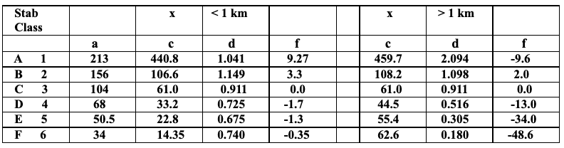
• In practice, \(\sigma_y(x)\) and \(\sigma_z(x)\) are fitted per stability class: e.g. \(\sigma_y = 34\,x^{0.894}\) (class F, \(x\) in km).

The derivation fixes the Gaussian shape; the data fix the widths.

References

References

Boussinesq, J. (1877). Essai sur la théorie des eaux courantes. Mémoires présentés par divers savants à l’Académie des Sciences, 23, 1–680.

Einstein, A. (1905). Über die von der molekularkinetischen Theorie der Wärme geforderte Bewegung von in ruhenden Flüssigkeiten suspendierten Teilchen. Annalen der Physik, 322(8), 549–560. https://doi.org/10.1002/andp.19053220806

Fick, A. (1855). Ueber Diffusion. Annalen der Physik, 170(1), 59–86. https://doi.org/10.1002/andp.18551700105

Pasquill, F. (1961). The estimation of the dispersion of windborne material. Meteorological Magazine, 90(1063), 33–49.

Taylor, G. I. (1922). Diffusion by continuous movements. Proceedings of the London Mathematical Society, s2-20(1), 196–212. https://doi.org/10.1112/plms/s2-20.1.196