Monte Carlo Error and Risk

---

Lecture 09

September 28, 2026

Overview

• Review of Last Class
• Confidence Intervals
• Dissolved Oxygen Example
• Justifying a Sample Size
• Probability vs. Risk
• Key Takeaways and Upcoming Schedule
• References

Review of Last Class

Monte Carlo Estimate and Error

Monte Carlo Principle: Estimate \(\mu = \mathbb{E}[Y] = \mathbb{E}[f(X)]\) using \[\tilde\mu_n = \frac{1}{n}\sum_{i=1}^n Y_i\dots.\]

This is an unbiased estimate, and \[\tilde\sigma_n = \frac{\sigma_Y}{\sqrt{n}}\]

is its standard error.

Derivation of MC Standard Error

\[\begin{aligned} \tilde{\sigma}_n^2 &= \text{Var}\left(\tilde{\mu}_n\right) \\ &= \text{Var}\left(\frac{1}{n}\sum_{i=1}^n Y_i\right) \\ &= \left(\frac{1}{n}\right)^2 \sum_{i=1}^n \text{Var}(Y_i) \\ &= \frac{1}{n^2} n \sigma_Y^2 = \frac{\sigma_Y^2}{n} \end{aligned}\]

Questions?

Text: VSRIKRISH to 22333

URL: https://pollev.com/vsrikrish

See Results

Confidence Intervals

MC Confidence Intervals

To get estimates of the error, we need to understand the distribution of errors.

The Central Limit Theorem says that sums of random variables converge to a Gaussian distribution.

Applying to the mean (which is effectively a sum):

\[\left\|\tilde{\mu}_n - \mu\right\| \to \mathcal{N}\left(0, \frac{\sigma_Y^2}{n}\right)\]

Confidence Intervals

We can use this large-\(n\) Gaussian approximation to get an \(\alpha\)-confidence interval.

\[\tilde\mu_n \pm \Phi^{-1}\left(1-\frac{\alpha}{2}\right)\frac{\sigma_Y}{\sqrt{n}}\]

For 95%: \[\tilde\mu_n \pm 1.96\frac{\sigma_Y}{\sqrt{n}}.\]

Reading a CI Correctly

A 95% CI is not “there is a 95% chance the true value is in this interval.” According to the frequentist interpretation of statistics, the true value is fixed.

For any given experiment, the “true value” is either in or out of the constructed interval.

The idea: if you repeated this whole experiment many times, about 95% of the intervals you’d construct would contain the true value.

Example: 95% CIs for N(0.4, 2)

# set up distribution
mean_true = 0.4
n_cis = 100 # number of CIs to compute
dist = Normal(mean_true, 2)

# use sample size of 100
samples = rand(dist, (100, n_cis))
# mapslices broadcasts over a matrix dimension, could also use a loop
sample_means = mapslices(mean, samples; dims=1)
sample_sd = mapslices(std, samples; dims=1) 
mc_sd = 1.96 * sample_sd / sqrt(100)
mc_ci = zeros(n_cis, 2) # preallocate
for i = 1:n_cis
    mc_ci[i, 1] = sample_means[i] - mc_sd[i]
    mc_ci[i, 2] = sample_means[i] + mc_sd[i]
end
# find which CIs contain the true value
ci_true = (mc_ci[:, 1] .< mean_true) .&& (mc_ci[:, 2] .> mean_true)
# compute percentage of CIs which contain the true value
ci_frac1 = 100 * sum(ci_true) ./ n_cis

# plot CIs
p1 = plot([mc_ci[1, :]], [1, 1], linewidth=3, color=:deepskyblue, label="95% Confidence Interval", title="Sample Size 100", yticks=:false, legend=:false)
for i = 2:n_cis
    if ci_true[i]
        plot!(p1, [mc_ci[i, :]], [i, i], linewidth=2, color=:deepskyblue, label=:false)
    else
        plot!(p1, [mc_ci[i, :]], [i, i], linewidth=2, color=:red, label=:false)
    end
end
vline!(p1, [mean_true], color=:black, linewidth=2, linestyle=:dash, label="True Value") # plot true value as a vertical line
xaxis!(p1, "Estimate")
plot!(p1, size=(500, 350)) # resize to fit slide

# use sample size of 1000
samples = rand(dist, (1000, n_cis))
# mapslices broadcasts over a matrix dimension, could also use a loop
sample_means = mapslices(mean, samples; dims=1)
sample_sd = mapslices(std, samples; dims=1) 
mc_sd = 1.96 * sample_sd / sqrt(1000)
mc_ci = zeros(n_cis, 2) # preallocate
for i = 1:n_cis
    mc_ci[i, 1] = sample_means[i] - mc_sd[i]
    mc_ci[i, 2] = sample_means[i] + mc_sd[i]
end
# find which CIs contain the true value
ci_true = (mc_ci[:, 1] .< mean_true) .&& (mc_ci[:, 2] .> mean_true)
# compute percentage of CIs which contain the true value
ci_frac2 = 100 * sum(ci_true) ./ n_cis

# plot CIs
p2 = plot([mc_ci[1, :]], [1, 1], linewidth=3, color=:deepskyblue, label="95% Confidence Interval", title="Sample Size 1,000", yticks=:false, legend=:false)
for i = 2:n_cis
    if ci_true[i]
        plot!(p2, [mc_ci[i, :]], [i, i], linewidth=2, color=:deepskyblue, label=:false)
    else
        plot!(p2, [mc_ci[i, :]], [i, i], linewidth=2, color=:red, label=:false)
    end
end
vline!(p2, [mean_true], color=:black, linewidth=2, linestyle=:dash, label="True Value") # plot true value as a vertical line
xaxis!(p2, "Estimate")
plot!(p2, size=(500, 350)) # resize to fit slide

display(p1)
display(p2)

(a) Sample Size 100

(b) Sample Size 1,000

Figure 1: Display of 95% confidence intervals

90% of the CIs contain the true value (left) vs. 93% (right)

Pseudorandomness and Seeds

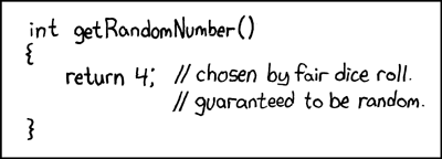
Random number generators are not really random — only pseudorandom, and deterministic given a seed.

Always set a seed. It’s how your results reproduce. But sometimes even that can go wrong…

XKCD 221: Random Number

Source: XKCD #221

MC Example: Dice

What is the probability of rolling 4 dice for a total of 19?

MC Example: Dice

function dice_roll_repeated(n_trials, n_dice)
    dice_dist = DiscreteUniform(1, 6) 
    roll_results = zeros(n_trials)
    for i=1:n_trials
        roll_results[i] = sum(rand(dice_dist, n_dice))
    end
    return roll_results
end

nsamp = 10_000
# roll four dice 10,000 times
rolls = dice_roll_repeated(nsamp, 4) 

# initialize storage for frequencies by sample length
avg_freq = zeros(length(rolls)) 
# initialize storage for standard error of estimate
std_freq = zeros(length(rolls))
# compute average frequencies of 19
avg_freq[1] = (rolls[1] == 19)
std_freq[1] = 0 # no standard error for the first sample

for i in 2:length(rolls)
    avg_freq[i] = (avg_freq[i-1] * (i-1) + (rolls[i] == 19)) / i
    std_freq[i] = std(rolls[1:i] .== 19) / sqrt(i)
end

plt = plot(
    avg_freq, ribbon=1.96 * std_freq,
    xlim = (1, nsamp),
    ylim = (0, 0.1),
    fillcolor=cb_blue,
    legend = :false,
    xlabel="Iteration",
    ylabel="Estimate",
    left_margin=10mm,
    bottom_margin=10mm,
    right_margin=10mm,
    color=:black,
    linewidth=3
)
plot!(size=(1200, 500))

hline!(plt, [0.0432], color="red", 
    linestyle=:dash) 

MC Example: Dice

After 10,000 iterations, the 95% confidence interval for the MC estimate is 4.4 \(\pm\) 0.4%.

Is this good enough? Should we keep going?

Dissolved Oxygen Example

What Is The Reliability of the System?

Or:

What is the probability that the minimum DO falls below a regulatory standard on a random day?

Sampling the Three Inputs

Input	Distribution (mg/L)
Mixed DO, \(C_0\)	\(\mathcal{N}(6.2, 0.5^2)\), at most 7
Mixed CBOD, \(B_0\)	\(\mathcal{N}(9, 1.5^2)\), at least 0
Mixed NBOD, \(N_0\)	\(\mathcal{N}(7, 1^2)\), at least 0

We draw them independently. CBOD and NBOD come from the same mixed effluent-river combination: is that reasonable?

Key Decision: What is the quantity we want to estimate?

Monte Carlo Simulation Code

do_params = let
    ka, kc, kn = 0.6, 0.4, 0.25   # reaeration, CBOD decay, NBOD decay [1/d]
    Cs, U = 7, 5                  # saturation DO [mg/L], velocity [km/d]
    L = 40                        # reach length [km]
    standard = 2.5                # DO standard [mg/L]
    (; ka, kc, kn, Cs, U, L, standard)
end

# The three uncertain inputs [mg/L]; truncation keeps every draw physical
mixed_DO = truncated(Normal(6.2, 0.5); upper=7)
mixed_CBOD = truncated(Normal(9, 1.5); lower=0)
mixed_NBOD = truncated(Normal(7, 1); lower=0)

function do_min(C0, B0, N0, params; dx=0.1)
    steps = Int(round(params.L / dx))
    C = zeros(steps + 1)
    C[1] = C0
    for i in 1:steps
        x = (i - 1) * dx
        C[i+1] = C[i] + dx * ((params.ka * (params.Cs - C[i]) - params.kc * B0 * exp(-params.kc * x / params.U)
                        - params.kn * N0 * exp(-params.kn * x / params.U)) / params.U)
    end
    return minimum(C)
end

# One Monte Carlo sample: draw all three inputs, then check the standard
function violates(params; dx=0.1)
    C0 = rand(mixed_DO)
    B0 = rand(mixed_CBOD)
    N0 = rand(mixed_NBOD)
    return do_min(C0, B0, N0, params; dx=dx) < params.standard
end

Monte Carlo Estimate By Sample

Random.seed!(1)
N = 20_000
draws = [violates(do_params) for _ in 1:N]
running_p = cumsum(draws) ./ (1:N)
running_se = zeros(N)
running_se[1] = 0 # no standard error for the first sample
for i in 2:N
    running_se[i] = std(draws[1:i]) / sqrt(i)
end

# Sample standard deviation of one draw, used later to predict the half-width for any n
draw_sd = std(draws)

p_mc = plot(1:N, running_p, ribbon=1.96 .* running_se, xscale=:log10,
    color=:black, linewidth=3, fillalpha=0.25, fillcolor=cb_blue,
    xlabel="Number of samples  n", ylabel="P(violation)", legend=false,
    ylims=(0, 1))
plot!(p_mc, size=(1100, 460), left_margin=12mm, right_margin=8mm,
    bottom_margin=12mm, top_margin=5mm)

Figure 2: Running Monte Carlo estimate of P(violation), with its 95% confidence band.

Evolution of Estimates and CI Over Simulation

\(n\)	estimate	95% CI
\(5\)	\(0.8\)	\([0.41, 1.19]\)
\(20\)	\(0.6\)	\([0.38, 0.82]\)
\(100\)	\(0.54\)	\([0.44, 0.64]\)
\(500\)	\(0.47\)	\([0.42, 0.51]\)
\(2000\)	\(0.49\)	\([0.47, 0.51]\)
\(20000\)	\(0.49\)	\([0.48, 0.49]\)

Key Considerations

But: these estimates and how they converge are entirely dependent on the choice of input distribution(s) (and whether or not they are correlated).

You need to make sure you can justify those choices, either from empirical data or some field convention (e.g. wind speeds using a Weibull distribution).

Justifying a Sample Size

Two Potential Sources of Error

Discretization

• pick \(\Delta t\) from a characteristic timescale
• halve it; see if the answer moves
• error scales linearly with \(\Delta t\)

Monte Carlo

• pick \(n\) from a target CI half-width
• double it; see if the estimate moves
• error scales as \(\sim 1/\sqrt{n}\)

Put Them in the Same Units

The two errors are not comparable until they describe the same quantity, the output of interest.

Here: Express both as the error in the violation probability.

• Discretization error: hold \(n\) and the seed fixed, vary \(\Delta x\)/\(\Delta t\), see how the probability moves.
• Sampling error: hold \(\Delta x\)/\(\Delta t\) fixed, and read the half-width \(1.96\, s_Y/\sqrt{n}\), where \(s_Y\) is the sample standard deviation of the draws.

Measuring the Grid Error

function violation_fraction(grid_step, sample_count, seed)
    Random.seed!(seed)
    violations = 0
    for _ in 1:sample_count
        if violates(do_params; dx=grid_step)
            violations += 1
        end
    end
    return violations / sample_count
end

grid_steps = [1, 0.5, 0.25, 0.1]
reference_p = violation_fraction(0.02, 3000, 99)

grid_estimates = zeros(length(grid_steps))
for i in 1:length(grid_steps)
    grid_estimates[i] = violation_fraction(grid_steps[i], 3000, 99)
end
grid_errors = abs.(grid_estimates .- reference_p)

\(\Delta x\) (km)	\(P\)	error vs. fine grid
\(1.0\)	\(0.67\)	\(0.18\)
\(0.5\)	\(0.57\)	\(0.08\)
\(0.25\)	\(0.53\)	\(0.04\)
\(0.1\)	\(0.5\)	\(0.01\)

Held fixed: \(n = 3{,}000\), seed 99. Reference: \(\Delta x = 0.02\) km.

Measuring the Sampling Error

Held fixed: \(\Delta x = 0.1\) km, with \(s_Y\) from the 20,000 draws on the Monte Carlo estimate slide. Varied: \(n\).

\(n\)	95% half-width
\(100\)	\(0.1\)
\(500\)	\(0.04\)
\(2000\)	\(0.02\)
\(8000\)	\(0.01\)

Where Should the Next Run Go?

Start from the settings we have been using, \(\Delta x = 0.1\) km and \(n = 2{,}000\). Each refinement doubles the cost of a run:

Refinement	Error removed
Halve \(\Delta x\) (0.1 → 0.05 km)	0.009 (measured)
Double \(n\) (2,000 → 4,000)	0.006 (predicted)

For the same cost, refining the grid removes about 1.5 times as much error.

It Depends on Where You Start

Which refinement removes more error for the same cost, and by how much?

Starting \(\Delta x\)	\(n = 100\)	\(n = 500\)	\(n = 2000\)	\(n = 8000\)
1 km	\(\Delta x\), 3.3×	\(\Delta x\), 7.5×	\(\Delta x\), 15×	\(\Delta x\), 29.9×
0.5 km	\(\Delta x\), 1.6×	\(\Delta x\), 3.7×	\(\Delta x\), 7.4×	\(\Delta x\), 14.8×
0.1 km	\(n\), 3.1×	\(n\), 1.4×	\(\Delta x\), 1.5×	\(\Delta x\), 2.9×

What Each Refinement Buys

Both refinements double the cost of a run. From the current settings:

• Halve \(\Delta x\): forward Euler is first order, so the grid error goes from \(e_{\Delta x}\) to \(e_{\Delta x}/2\). You remove \(\tfrac{1}{2}\,e_{\Delta x}\).
• Double \(n\): the half-width \(h_n = 1.96\,s_Y/\sqrt{n}\) goes from \(h_n\) to \(h_n/\sqrt{2}\). You remove \(h_n - h_n/\sqrt{2} \approx 0.29\,h_n\).

When to Add Samples

Doubling \(n\) removes more error than halving \(\Delta x\) when

\[(1 - 1/\sqrt{2})\,h_n > \tfrac{1}{2}\,e_{\Delta x} \iff h_n > (1 + 1/\sqrt{2})\,e_{\Delta x} \approx 1.7\,e_{\Delta x}.\]

Unless the Monte Carlo half-width is at least 1.7 times the grid error, the grid is the lowest-hanging fruit.

At \(\Delta x = 0.1\) km and \(n = 2{,}000\): \(h_n =\) 0.022 and \(1.7\,e_{\Delta x} =\) 0.025, so halve \(\Delta x\).

How To Report Error

Your confidence interval is computed from \(n\) alone. It doesn’t reflect the discretization error.

So a report that says \(P =\) 0.49 \(\pm\) 0.02 leaves out a grid error of about 0.015 at \(\Delta x = 0.1\) km, most of the size of the interval itself.

Only reporting the Monte Carlo CI if there is also discretization error can mislead!

Know Your Error Tolerance

Ultimately, at some point chasing more error reduction does not help your analysis.

Here: suppose the river may violate the standard on at most 10% of days (a hypothetical tolerance).

• \(P =\) 0.49 \(\pm\) 0.04 (sampling plus grid error): 0.39 above the tolerance.
• Halving \(\Delta x\) would move it by 0.009.

When Would the Error Matter?

Against a 10% tolerance, even the coarsest grid (\(\Delta x = 1\) km, \(P =\) 0.67) gives the same answer: the river fails.

If the tolerance were 50%, \(P =\) 0.49 \(\pm\) 0.04 would straddle it, and refining would decide the answer.

Set the tolerance from the decision before choosing \(\Delta x\) and \(n\).

Probability vs. Risk

What Risk Means

The Society for Risk Analysis definition:

“risk” involves uncertainty about the effects/implications of an activity with respect to something that humans value (such as health, well-being, wealth, property or the environment), often focusing on negative, undesirable consequences.

Risk Is Not Probability

“Risk” is not just another word for probability. It involves:

• uncertainty;
• undesirable outcomes;
• effects, not just the events themselves.

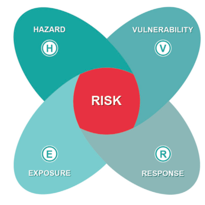
Components of Risk

Several things combine to produce risk:

• Probability of a hazard;
• Exposure to that hazard;
• Vulnerability to the outcomes;
• Socioeconomic responses.

Overview of the Components of Risk

Source: Simpson et al. (2021)

Our DO Model Contains Only One of Four

\(P(\text{DO} < 2.5)\) is a hazard statistic, and nothing more.

• Who is exposed? What residents, intakes, ecosystems?
• How vulnerable are they? A brief reduction in DO matters differently to a trout community than to an industrial intake.
• What is the response? A warning system might cause the effluent release to change.

Key Takeaways and Upcoming Schedule

Key Takeaways

• A confidence interval describes the procedure, not the one interval you happened to construct.
• Sample size needs justification: check if the estimate is stable and make sure the CI half-width is small enough.
• Discretization error and Monte Carlo error are included in every MC estimate you produce using a discretized simulation model. They fall at different rates: include both and focus computation where the potential for error reduction is greatest.

Next Classes

Wednesday/Monday: Gaussian Plumes and 2D Simulation

Assessments

Quiz 2: Monday, October 5, covering discretization, convergence, Streeter-Phelps, and Monte Carlo, including confidence intervals and risk.

Homework 4: Due Thursday, October 8.

Mini-Project 1: Due Thursday, October 22.

Project Proposal: Due Friday, October 16. See website for guidelines.

References

References