Uncertainty, Probability, and Monte Carlo

---

Lecture 08

September 23, 2026

Overview

• Review of Last Class
• Uncertainty and Probability
• Monte Carlo Simulation
• How Uncertain is the Estimate?
• Key Takeaways and Upcoming Schedule
• References

Review of Last Class

Dissolved Oxygen and Streeter-Phelps

• Dissolved Oxygen: Critical for aquatic life/ecosystem health
• Depleted by decomposition of organic matter/waste, often regulated
• Derived Streeter-Phelps equation: produces sag curve due to competition between reaeration and decomposition of CBOD and NBOD.

Questions?

Text: VSRIKRISH to 22333

URL: https://pollev.com/vsrikrish

See Results

Uncertainty and Probability

Where Does Uncertainty Come From?

Uncertainty can come from several sources:

• Stochastic models (internal randomness)
• Uncertain external conditions (forcings)
• Uncertain parameters
• Uncertain model dynamics from different specifications/neglecting processes

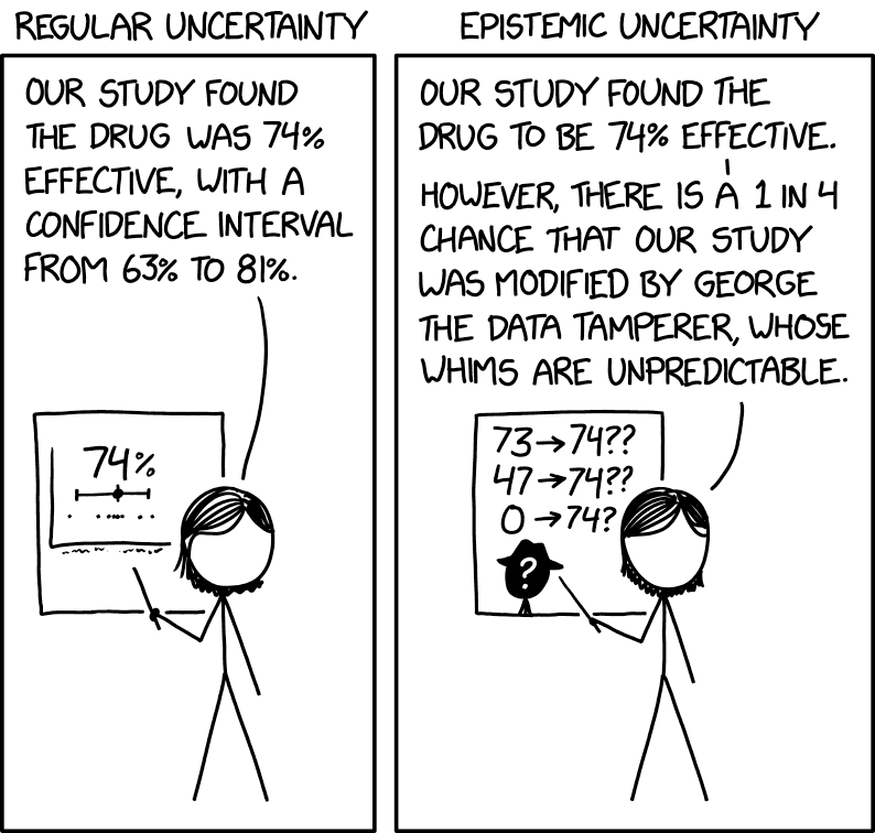
Two Kinds of Uncertainty

• Aleatory uncertainty: “Truly” random processes/fluctuations.
• Epistemic uncertainty: From lack of knowledge.

Aleatory vs epistemic uncertainty

Source: XKCD 2440

Aleatory vs. Epistemic Examples

Would more data or study reduce the uncertainty? If so, it is epistemic. If it is unpredictable randomness, it is aleatory.

Aleatory	Epistemic
The next roll of a die	Whether the die is loaded
When your light bulb fails	The bulb model’s lifespan
Next spring’s peak flow	The 100-year flood
Tomorrow’s commute traffic	Next week’s quiz questions

Random Variables

A random variable is a quantity whose value we do not know. Its distribution describes how plausible each possible value is.

Discrete: values you can list, like storms per year.

Probability mass function: \(p(x) = \mathbb{P}(X = x)\)

Continuous: any value in a range, like CBOD load.

Probability density function: \(\mathbb{P}(a < X < b) = \int_a^b f(x)\,dx\)

What Is a Probability Distribution?

A probability distribution assigns probabilities to the possible outcomes of a random variable, following three rules:

1. \(\mathbb{P}(A) \geq 0\) for any event \(A\)
2. \(\mathbb{P}(\text{some outcome occurs}) = 1\)
3. \(\mathbb{P}(A \cup B) = \mathbb{P}(A) + \mathbb{P}(B)\) if \(A\) and \(B\) cannot both happen

Notation: \(X \sim \mathcal{D}\) means \(X\) follows \(\mathcal{D}\), e.g. \(B_0 \sim \mathcal{N}(9, 1.5^2)\).

Density and Cumulative Probability

A probability distribution \(\mathcal{D}\) is described using two equivalent specifications:

• Probability Density Function (PDF) \(f_\mathcal{D}(x)\): how concentrated is the probability at \(x\).
• Cumulative Distribution Function (CDF) \(F_\mathcal{D}(x) = \int_{-\infty}^x f_\mathcal{D}(u)\,du\): what is the total probability at or below \(x\).

CDF vs. PDF

example_dist = TDist(4)
x_values = -5:0.01:5
level = 0.25
cut = quantile(example_dist, level)

p_pdf = plot(x_values, pdf.(example_dist, x_values), color=:black, linewidth=4,
    xlabel=L"x", ylabel="Density", legend=false)
shaded = -5:0.01:cut
plot!(p_pdf, shaded, pdf.(example_dist, shaded), fillrange=zeros(length(shaded)),
    fillalpha=0.35, color=cb_blue, linewidth=0)

p_cdf = plot(x_values, cdf.(example_dist, x_values), color=:black, linewidth=4,
    xlabel=L"x", ylabel="Cumulative probability", legend=false)
plot!(p_cdf, [-5, cut], [level, level], color=cb_vermillion, linewidth=3, linestyle=:dash)
plot!(p_cdf, [cut, cut], [0, level], color=cb_vermillion, linewidth=3, linestyle=:dash)

plot(p_pdf, p_cdf, layout=(1, 2), size=(1200, 450), left_margin=10mm,
    bottom_margin=10mm)

Figure 1: The shaded area under the density is the height of the cumulative curve. Both panels show the same quarter of the probability.

Quantiles

The quantile function is the inverse of the CDF:

\[q(\alpha) = F^{-1}_\mathcal{D}(\alpha), \qquad\text{so}\qquad x_0 = q(\alpha) \iff \mathbb{P}(X < x_0) = \alpha.\]

• CDF: for a given \(x_0\), what is \(\mathcal{P}(X \leq x_0)\)?
• Quantile: for a given \(0 \leq \alpha \leq 1\), what value \(x_0\) has \(\mathcal{P}(X \leq x_0) = \alpha\)?

Independence

Two events are independent if knowing one happened tells you nothing about the other:

\[\mathbb{P}(A \cap B) = \mathbb{P}(A)\,\mathbb{P}(B)\]

Expectation and Variance

\[\begin{aligned} \mathbb{E}[X] &= \int x f(x)\,dx \\ \text{Var}(X) &= \mathbb{E}\left[(X - \mathbb{E}[X])^2\right] \end{aligned}\]

Rules for Expectation and Variance

For constants \(a\) and \(b\) and random variables \(X\) and \(Y\):

\[\begin{aligned} \mathbb{E}[aX + b] &= a\,\mathbb{E}[X] + b \\ \text{Var}(aX + b) &= a^2\,\text{Var}(X) \\ \mathbb{E}[X + Y] &= \mathbb{E}[X] + \mathbb{E}[Y] \\ \end{aligned}\]

If \(X\) and \(Y\) are independent: \[\text{Var}(X + Y) = \text{Var}(X) + \text{Var}(Y)\]

The Average of a Function Is Not the Function of the Average

\[\mathbb{E}[h(B_0)] = h(\mathbb{E}[B_0])\ \text{if and only if}\ h\ \text{is linear}.\]

Which of these do we want?

Distributions Are Assumptions

Specifying a distribution is making an assumption about the probability model producing observations.

There are defaults. If your data is:

• Continuous and fat-tailed? Cauchy distribution
• Continuous and bounded? Beta distribution
• Sums of positive random variables? Gamma or Normal distribution

Common Distributions

Distribution	Use it when
Uniform	Every value in a range equally likely
Normal	Symmetric about a typical value
LogNormal	Positive and right-skewed
Bernoulli	A yes/no event

Selecting a Distribution

A distribution implicitly answers questions like:

• What is the most probable event? How much more likely is it than the others?
• Are larger or smaller events more, less, or equally probable?
• How probable are extreme events?
• Are different events correlated, or are they independent?

Distribution Tails

The tails represent the probability of high-impact outcomes.

Small changes to these (low) probabilities can greatly influence risk.

x = range(-5, 10, length=200)
p_tails = plot(x, pdf.(Cauchy(), x), linewidth=3, color=cb_vermillion,
    linestyle=:dash, yaxis=false, yticks=false, label="Cauchy", xlabel="Value",
    legend=:topright)
plot!(p_tails, x, pdf.(Normal(), x), linewidth=3, color=cb_blue, label="Normal")
xf = x[x.>1.75]
plot!(p_tails, xf, pdf.(Cauchy(), xf), fillrange=pdf.(Normal(), xf),
    fillcolor=cb_vermillion, fillalpha=0.25, label=nothing, linecolor=nothing)
plot!(p_tails, size=(550, 420), left_margin=10mm, bottom_margin=10mm)

Figure 2: Comparison of Cauchy and Normal tails.

“What Distribution Should I Use?”

There is no right answer, no matter what a statistical test tells you.

• What assumptions are justifiable? Think about tails, symmetry, skew.
• What information do you actually have?

Choosing \(B_0\)’s Distribution

For the CBOD load: not too far from a typical value, symmetric-ish, occasionally larger or smaller by a moderate amount, never negative in reality (though the Normal doesn’t know that).

\[B_0 \sim \mathcal{N}(9,\ 1.5^2)\ \text{mg/L}\]

Perhaps use a truncated Normal to eliminate possibility of negatives.

Standards Are Written as Probabilities

Design and regulatory standards are almost never stated as “never fails.” They are usually stated as frequencies.

For example:

Levees in the United States are supposed to only fail at “once in 100 years” — or, equivalently, to have at most a 1% chance of failure in any given year.

Exceedance Probability

The probability that a quantity is worse than some threshold \(x^*\):

\[p = \mathbb{P}(X > x^*) = 1 - F_\mathcal{D}(x^*)\]

It is the complement of the CDF.

Return Periods

The return period is its reciprocal:

\[T = \frac{1}{p}\]

A 1% annual exceedance probability is a 100-year event. The two say exactly the same thing in different units.

How Often Does An Extreme Occur?

A “100-year event” does not mean one per century, or that you are safe for 99 years after one happens.

If years are independent, the chance of at least one in a 30-year design life is \[1 - (1 - 0.01)^{30} \approx 26\%.\] Better than one in four, over the life of the structure.

What a Return Period Assumes

• Each year is an independent draw.
• The distribution is not changing — the same \(F\) next decade as last.
• If it is changing, the return period is conditional on the scenario driving the change.

Where Would We Get \(F\)?

Exceedance probability is \(1 - F(x^*)\). That is easy when you know \(F\).

For many systems, you do not. Outcomes of interest may be the output of a non-linear system with multiple inputs.

In that case, we need a simulation-based approach to estimate expectations or exceedance probabilities.

Monte Carlo Simulation

What Is Monte Carlo?

Monte Carlo simulation: propagate random samples through a model to estimate a value — usually an expectation or a probability.

The Monte Carlo Principle

Goal: estimate \(\mathbb{E}_f[h(x)]\) for \(x \sim f(x)\).

Sample \(x^1, \ldots, x^N \sim f(x)\) and estimate

\[\mathbb{E}_f[h(x)] = \int_{x\in X} h(x)f(x)\,dx \approx \frac{1}{N}\sum_{n=1}^N h(x^n)\]

A probability is just a special case: \(h(x) = \mathbb{1}[\text{event}]\), and the average becomes a frequency.

Example: Estimating \(\pi\)

Sample points uniformly in a square; the fraction landing in the inscribed circle estimates

\[\frac{\text{Area of Circle}}{\text{Area of Square}} = \frac{\pi}{4}\]

using Logging

Random.seed!(4750)
sample_count = 3000
points = rand(Uniform(-1, 1), (sample_count, 2))
inside = [points[i, 1]^2 + points[i, 2]^2 < 1 for i in 1:sample_count]
running_estimate = [4 * mean(inside[1:i]) for i in 1:sample_count]

circle_angles = range(0, 2π, length=500)
batch_size = 100

# Each frame redraws everything drawn so far, 100 more samples at a time.
animation = @animate for shown_count in batch_size:batch_size:sample_count
    shown_points = points[1:shown_count, :]
    shown_inside = inside[1:shown_count]

    p_square = plot(cos.(circle_angles), sin.(circle_angles), color=:black, linewidth=1,
        xlims=(-1, 1), ylims=(-1, 1), xticks=[-1, 0, 1], yticks=[-1, 0, 1],
        aspect_ratio=1, legend=false)
    scatter!(p_square, shown_points[shown_inside, 1], shown_points[shown_inside, 2],
        color=cb_blue, markershape=:x, markersize=3)
    scatter!(p_square, shown_points[.!shown_inside, 1], shown_points[.!shown_inside, 2],
        color=cb_vermillion, markershape=:x, markersize=3)

    p_estimate = plot(1:shown_count, running_estimate[1:shown_count], color=:black,
        linewidth=3, xlims=(1, sample_count), ylims=(2.8, 3.5), legend=false,
        xlabel="Number of samples", ylabel="Estimate")
    hline!(p_estimate, [π], color=cb_green, linestyle=:dash, linewidth=2)

    plot(p_square, p_estimate, layout=grid(2, 1, heights=[3/4, 1/4]), size=(600, 550),
        right_margin=8mm)
end

# gif() prints a "saved animation" message; this keeps it off the slide.
Logging.disable_logging(Logging.Info)
gif(animation, "figures/mc_pi.gif", fps=2)

Figure 3: Points are revealed 100 at a time. Blue land inside the circle, vermillion outside, and the estimate settles toward π (dashed).

How Uncertain is the Estimate?

Monte Carlo Estimates Are Random

\(Y_i\) is a random sample, so \(\tilde{\mu}_n = \frac{1}{n}\sum_{i=1}^n Y_i\) is a random variable.

This raises the question: on average, how right or wrong is the estimate?

Bias of a statistic \(T\) used to estimate a “true” value \(T_0\): \(\mathbb{E}[T] - T_0\).

MC Estimates Is Unbiased

Provided the mean of \(Y\) exists and its variance is finite,

\[\mathbb{E}[\tilde{\mu}_n] = \frac{1}{n}\sum_{i=1}^n \mathbb{E}[Y_i] = \frac{1}{n}\, n\, \mu = \mu.\]

Averaged over many sets of samples, the estimate is correct. That is a statement about the procedure, not about the run you just did.

Monte Carlo Convergence

What are the convergence properties of any given MC run?

If \(Y\) is a random variable whose expectation exists, and \(Y_1, \ldots, Y_n\) are independent and identically distributed, then by the weak law of large numbers

\[\lim_{n \to \infty} \mathbb{P}\left(\tilde{\mu}_n - \mu \leq \varepsilon\right) = 1\]

for any \(\varepsilon > 0\).

Monte Carlo Error

The variance of the estimator is

\[\text{Var}(\tilde\mu_n) = \frac{\sigma_Y^2}{n} \qquad\Longrightarrow\qquad \text{standard error } \tilde\sigma_n = \frac{\sigma_Y}{\sqrt{n}}\]

In practice: replace \(\sigma_Y\) with the sample standard deviation \(\sqrt{\text{Var}(Y_i)}\).

Implications of Monte Carlo Error

To cut the error by 10×, you need 100× more samples. Monte Carlo converges at order \(\sqrt{n}\).

Monte Carlo is an extremely bad method. It should only be used when all alternative methods are worse.

— Sokal, Monte Carlo Methods in Statistical Mechanics, 1996

Key Takeaways and Upcoming Schedule

Key Takeaways

• Uncertainty comes from stochastic models, forcings, parameters, and model structure itself — and choosing a distribution is a modeling assumption, not a neutral default.
• The average outcome is not the outcome at the average input. For a nonlinear model those differ, which is why we sample rather than run once at the mean.
• An exceedance probability is \(1 - F(x^*)\), and a return period is its reciprocal. Neither means “once per century.”
• Monte Carlo estimates are unbiased and the law of large numbers says they converge — but the standard error shrinks only as \(1/\sqrt{n}\).

Next Classes

Monday: Confidence intervals, then applying Monte Carlo to the DO model and how to justify a sample size for your own work.

The probability tutorial covers today’s review in more depth, with Julia examples.

Assessments

Homework 3: Due tomorrow at 9pm.

Mini-Project 1: Assigned today, due Thursday, October 22.

References

References