sp_params = let
    ka, kc, kn = 0.6, 0.4, 0.25    # reaeration, CBOD decay, NBOD decay   [1/d]
    B0, N0 = 9.0, 7.0               # initial CBOD, NBOD                  [mg/L]
    Cs, U = 7.0, 5.0                 # saturation DO [mg/L], velocity [km/d]
    (; ka, kc, kn, B0, N0, Cs, U)
end
C0 = 6.2   # initial DO deficit-state [mg/L] -- a scenario choice, not a model constant

do_change(C, x, params) =
    (params.ka * (params.Cs - C) - params.kc * params.B0 * exp(-params.kc * x / params.U)
     - params.kn * params.N0 * exp(-params.kn * x / params.U)) / params.U

function simulate_do(C_ic, L, Δx, params)
    steps = Int(round(L / Δx))
    C = zeros(steps + 1)
    C[1] = C_ic
    for i in 1:steps
        C[i+1] = C[i] + Δx * do_change(C[i], (i - 1) * Δx, params)
    end
    return C
endStreeter-Phelps and Dissolved Oxygen
Lecture 07
September 16, 2026
Review of Last Class
Numerical Solutions Are Samples on a Grid
Track the state at a sequence of times \(t_0, t_1, t_2, \ldots\) and use the model to advance from one to the next:
\[X(t + \Delta t) = X(t) + \underbrace{\Delta X_t}_{\text{derived from } dX/dt}\]
The grid is a choice we make, not a property of the system. Everything we report is read off those samples.
Forward Euler Is First Order
Evaluate the rate at the state we already know:
\[\bbox[5pt, border: 3px solid red]{X(t+\Delta t) = X(t) + \Delta t\, f\left(X(t)\right)}\]
- Local error per step is \(O(\Delta t^2)\); we take \(T/\Delta t\) steps, so global error is \(O(\Delta t)\).
- Practically: halve \(\Delta t\), halve the error.
- On log-log axes, the slope of error against \(\Delta t\) is that order.
How We Justified a Step Size
Where to start
The characteristic timescale \(1/|\text{rate}|\) of the fastest process in the model. \(\Delta t\) must sit well inside it.
When to stop
Name a scalar quantity of interest, halve \(\Delta t\) until it stops moving, and report what that changed.
Neither step is optional: the timescale tells you where to begin, the refinement tells you when you are done.
Questions?

Text: VSRIKRISH to 22333
Modeling Dissolved Oxygen
Dissolved Oxygen
Dissolved oxygen (DO) is the free, non-compound oxygen present in water.
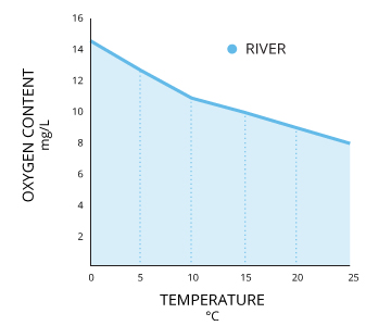
Freshwater can only hold small amounts, and this capacity is regulated by temperature.
Source: fondriest.com
Dissolved Oxygen and Life
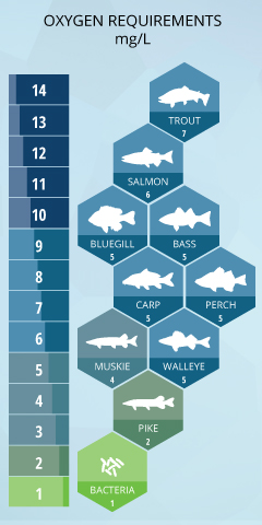
DO is essential for aquatic life.
Hypoxia occurs when DO levels are \(< 2\) mg/L.
Source: fondriest.com
Impact of Paris on Seine DO, 1874
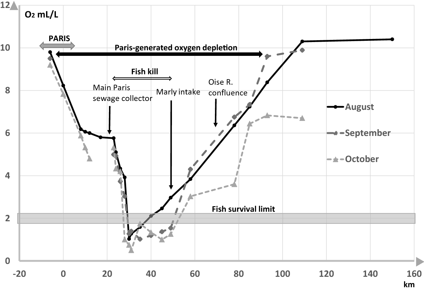
Dissolved Oxygen Downstream of Paris, 1874
Source: Dmitrieva, T., et al. (2018). https://doi.org/10.1007/s12685-018-0216-7
DO Regulatory Standards
Objective: Keep DO above the regulatory standard.
In NY (via Westlaw):
- DO levels may not fall below 3 mg/L
- DO may not be below 4.8 mg/L for an extended period
Oxygen Balance in Rivers and Streams
Biochemical Oxygen Demand (BOD)
Oxygen used by microbes during aerobic decomposition of organic matter: \[\text{Organic Matter} + \text{O}_2 \rightarrow \text{CO}_2 + \text{H}_2\text{O} + \text{NO}_3 + \text{SO}_2 + \text{Residuals}\]
We track two kinds: Carbonaceous BOD (CBOD) from carbon compounds, and Nitrogenous BOD (NBOD) from nitrogen compounds.
Modeling DO
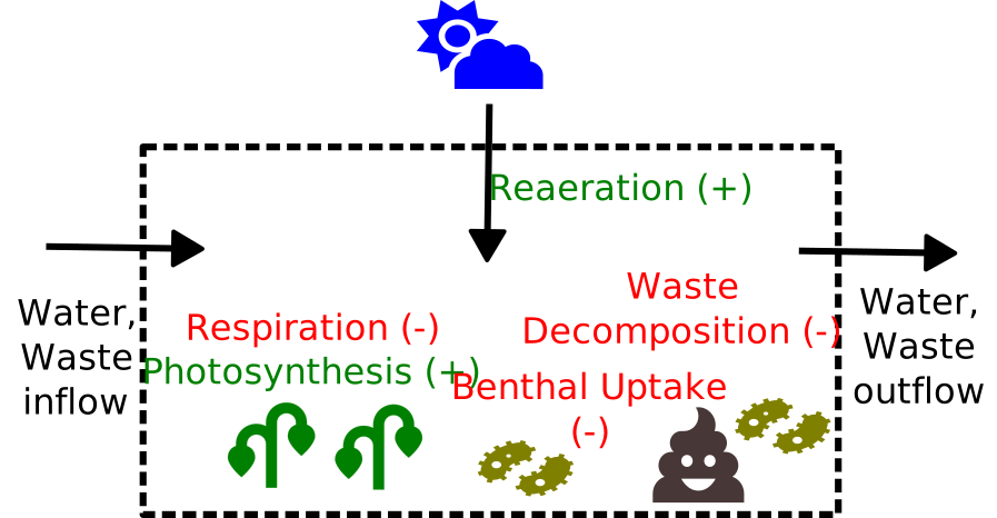
We track the mass balance in terms of rates, following an element of water as it moves downstream.
DO Mass Balance
Let \(U\) be the river velocity (km/d), \(x\) the distance downstream from a release site, and \(C(x)\) the DO concentration at \(x\) (mg/L):
\[\begin{aligned} U\frac{dC}{dx} &= \Delta\ \text{DO} = \text{Reaeration} + \text{Photosynthesis} - \text{Respiration} \\ &\qquad - \text{Benthal Uptake} - \text{CBOD} - \text{NBOD} \end{aligned}\]
BOD Oxygen Uptake
Deoxygenation from waste decomposition is first-order. In time: \(M = M_0 e^{-kt}\).
Our equation is in distance, so substitute \(t = x/U\):
\[B(x) = B_0 e^{-k_c x/U} \qquad\qquad N(x) = N_0 e^{-k_n x/U}\]
where \(k_c\), \(k_n\) are the CBOD and NBOD decay rates.
Putting It Together
Reaeration is proportional to the deficit from saturation, \(k_a(C_s - C)\). Photosynthesis (\(P\)), respiration (\(R\)), and benthal uptake (\(S_B\)) are usually measured and treated as constants:
\[\begin{aligned} U\frac{dC}{dx} &= k_a(C_s - C) + P - R - S_B \\ &\qquad - k_cB_0e^{-k_cx/U} - k_nN_0e^{-k_nx/U} \end{aligned}\]
Why Discretize an Equation You Can Solve?
Analytic Solution (Streeter-Phelps)
\[\begin{aligned} C(x) &= C_s(1-\alpha_1) + C_0\alpha_1 - B_0\alpha_2 - N_0\alpha_3 + \left(\frac{P-R-S_B}{k_a}\right)(1-\alpha_1) \\[0.25em] \alpha_1 &= \exp\left(\frac{-k_ax}{U}\right) \\[0.25em] \alpha_2 &= \left(\frac{k_c}{k_a-k_c}\right)\left[\exp\left(\frac{-k_cx}{U}\right) - \exp\left(\frac{-k_ax}{U}\right)\right] \\[0.25em] \alpha_3 &= \left(\frac{k_n}{k_a-k_n}\right)\left[\exp\left(\frac{-k_nx}{U}\right) - \exp\left(\frac{-k_ax}{U}\right)\right] \end{aligned}\]
What Assumptions Did We Make?
- \(U\), \(k_a\), \(k_c\), \(k_n\) are constant along the whole reach.
- \(P\), \(R\), \(S_B\) are constant (often zero).
- A single, steady release at \(x = 0\).
Two Reasons to Discretize Anyway
- Simplifies solving: each closed form makes its own assumptions — this one divides by \(k_a - k_c\) and \(k_a - k_n\), so equal rates need a separate formula (appendix). Change the kinetics and you re-derive from scratch. Forward Euler does not care.
- Conditions change as a parcel travels — temperature driving \(k_a\) through the day, changing \(U\), or dispersion mixing neighbouring parcels. Then no single closed form covers the trip.
When Don’t You Need To Discretize
- Multiple discharges: chain closed-form segments end to end, using one segment’s output as the next segment’s inlet condition. No discretization needed.
- A \(B_0\) that varies over time: each parcel still meets constant conditions on its way down, so it gets the same closed form — just started from the load released when it left.
Discretizing Anyway
Numerical Solution
What is the discretized version of the DO ODE?
\[ \begin{aligned} C(x + \Delta x) &= C(x) + \frac{\Delta x}{U}\Bigl[k_a (C_s - C(x)) + P - R - S_B \\ &\quad - k_cB_0\exp\left(\frac{-k_cx}{U}\right) - k_n N_0\exp\left(\frac{-k_nx}{U}\right)\Bigr] \end{aligned} \]
Code for Discretized Model
The Sag Curve
Code
L = 40.0
p_sag = plot(xlabel="Distance downstream  [km]", ylabel="DO  [mg/L]", legend=:bottomright)
plot!(p_sag, 0:0.002:L, simulate_do(C0, L, 0.002, sp_params), color=:black,
    linewidth=5, label="reference (Δx = 0.002)")
for (Δx, col) in zip([2.0, 1.0, 0.5], [cb_vermillion, cb_orange, cb_blue])
    plot!(p_sag, 0:Δx:L, simulate_do(C0, L, Δx, sp_params), color=col,
        linewidth=3, linestyle=:dash, markershape=:circle, markersize=4, label="Δx = $Δx")
end
hline!(p_sag, [2.5], color=cb_green, linewidth=3, linestyle=:dot, label="standard: 2.5 mg/L")
plot!(p_sag, size=(1100, 450), left_margin=12mm, right_margin=8mm,
bottom_margin=12mm, top_margin=5mm)Why Is There a Sag At All?
Code
# The closed-form solution is a sum of three pieces. Write each one out
# separately so we can plot them.

# Reaeration acting alone: DO relaxes from its starting value toward
# saturation. This piece only ever rises.
function reaeration_only(distance, params)
    reaeration = exp(-params.ka * distance / params.U)
    return params.Cs * (1 - reaeration) + C0 * reaeration
end

# Oxygen consumed by carbonaceous BOD. It is zero at the effluent (no time to
# act yet) and returns to zero once the CBOD is used up, so it must dip in
# between.
function cbod_drawdown(distance, params)
    reaeration = exp(-params.ka * distance / params.U)
    cbod_left  = exp(-params.kc * distance / params.U)
    return -params.B0 * (params.kc / (params.ka - params.kc)) * (cbod_left - reaeration)
end

# Same shape for nitrogenous BOD, but slower and shallower.
function nbod_drawdown(distance, params)
    reaeration = exp(-params.ka * distance / params.U)
    nbod_left  = exp(-params.kn * distance / params.U)
    return -params.N0 * (params.kn / (params.ka - params.kn)) * (nbod_left - reaeration)
end

distances     = 0:0.05:L
recovery_part = [reaeration_only(x, sp_params) for x in distances]
cbod_part     = [cbod_drawdown(x, sp_params) for x in distances]
nbod_part     = [nbod_drawdown(x, sp_params) for x in distances]
total_DO      = [recovery_part[i] + cbod_part[i] + nbod_part[i] for i in 1:length(distances)]

critical_point = distances[argmin(total_DO)]

p_comp = plot(xlabel="Distance downstream  [km]", ylabel="Contribution to DO  [mg/L]",
    legend=:outerright, ylims=(-4, 8))
hline!(p_comp, [0], color=:grey, linewidth=1, label=nothing)
plot!(p_comp, distances, recovery_part, color=cb_blue, linewidth=3,
    linestyle=:dash, label="reaeration alone")
plot!(p_comp, distances, cbod_part, color=cb_vermillion, linewidth=3,
    linestyle=:dashdot, label="CBOD drawdown")
plot!(p_comp, distances, nbod_part, color=cb_orange, linewidth=3,
    linestyle=:dot, label="NBOD drawdown")
plot!(p_comp, distances, total_DO, color=:black, linewidth=5, label="sum = DO")
vline!(p_comp, [critical_point], color=:grey, linewidth=2, linestyle=:dot, label=nothing)
annotate!(p_comp, critical_point + 1.0, -3.2,
    text("critical point\n$(round(critical_point, digits=1)) km", 14, :left))
plot!(p_comp, size=(1100, 450), left_margin=12mm, right_margin=8mm,
bottom_margin=12mm, top_margin=5mm)Impact of Step Size
| \(\Delta x\) (km) | minimum DO (mg/L) |
|---|---|
| \(4.0\) | \(1.3\) |
| \(2.0\) | \(2.0\) |
| \(1.0\) | \(2.3\) |
| \(0.5\) | \(2.4\) |
| \(0.25\) | \(2.5\) |
| \(0.125\) | \(2.5\) |
Does It Converge at First Order?
Code
Δxs = [4.0, 2.0, 1.0, 0.5, 0.25, 0.125, 0.0625]
min_ref = minimum(simulate_do(C0, L, 0.001, sp_params))
errs = [abs(minimum(simulate_do(C0, L, Δx, sp_params)) - min_ref) for Δx in Δxs]
orders = [round(log2(errs[i] / errs[i+1]), digits=2) for i in 1:length(errs)-1]

p_doconv = plot(Δxs, errs, xscale=:log10, yscale=:log10, markershape=:circle,
    markersize=7, color=cb_vermillion, linewidth=3, label="forward Euler",
    xlabel="Δx  [km]", ylabel="error in minimum DO  [mg/L]", legend=:bottomright)
plot!(p_doconv, Δxs, errs[1] .* (Δxs ./ Δxs[1]), color=:black, linewidth=2,
    linestyle=:dash, label="slope 1")
plot!(p_doconv, size=(1000, 430), left_margin=12mm, right_margin=8mm,
bottom_margin=12mm, top_margin=5mm)Multiple Discharges
Three Plants on One River
Each effluent mixes with the river; between effluents the closed form applies unchanged.
Note: No discretization needed — chain the segments by treating each stretch between each effluent as a “box” with a new initial condition, then using the closed form solution.
The Combined Sag Curve
Code
# Conditions in the river upstream of the first plant (clean water)
river_flow = 1.0e5      # m³/d
river_DO   = 6.8        # mg/L
river_CBOD = 0.0        # mg/L
river_NBOD = 0.0        # mg/L

# One entry per plant, in order going downstream
plant_location = [0.0, 18.0, 36.0]      # km
plant_flow     = [1.5e4, 1.5e4, 1.5e4]  # m³/d
plant_DO       = [1.0, 1.0, 1.0]        # mg/L
plant_CBOD     = [55.0, 50.0, 65.0]     # mg/L
plant_NBOD     = [33.0, 30.0, 39.0]     # mg/L

# Streeter-Phelps: DO after travelling `distance` down a stretch that begins
# with the given DO, CBOD, and NBOD.
function do_downstream(distance, DO_start, CBOD_start, NBOD_start, params)
    reaeration = exp(-params.ka * distance / params.U)
    cbod_left  = exp(-params.kc * distance / params.U)
    nbod_left  = exp(-params.kn * distance / params.U)

    recovery = params.Cs * (1 - reaeration) + DO_start * reaeration
    cbod_sag = CBOD_start * (params.kc / (params.ka - params.kc)) * (cbod_left - reaeration)
    nbod_sag = NBOD_start * (params.kn / (params.ka - params.kn)) * (nbod_left - reaeration)

    return recovery - cbod_sag - nbod_sag
end

# Each stretch below a plant is a "box": mix the effluent in to get the box's
# starting condition, then apply the closed form within the box.
function simulate_river(x_grid, location, flow, effluent_DO, effluent_CBOD, effluent_NBOD, params)
    DO = zeros(length(x_grid))

    # State of the water entering the current box
    current_flow = river_flow
    DO_in   = river_DO
    CBOD_in = river_CBOD
    NBOD_in = river_NBOD

    # Water upstream of the first plant is clean, so it relaxes toward saturation
    for i in 1:length(x_grid)
        if x_grid[i] < location[1]
            DO[i] = do_downstream(x_grid[i] - x_grid[1], river_DO, river_CBOD, river_NBOD, params)
        end
    end

    # Carry the clean river down to the first plant
    distance = location[1] - x_grid[1]
    DO_in   = do_downstream(distance, DO_in, CBOD_in, NBOD_in, params)
    CBOD_in = CBOD_in * exp(-params.kc * distance / params.U)
    NBOD_in = NBOD_in * exp(-params.kn * distance / params.U)

    for plant in 1:length(location)
        # Carry the river from the previous plant down to this one
        if plant > 1
            distance = location[plant] - location[plant-1]
            DO_in   = do_downstream(distance, DO_in, CBOD_in, NBOD_in, params)
            CBOD_in = CBOD_in * exp(-params.kc * distance / params.U)
            NBOD_in = NBOD_in * exp(-params.kn * distance / params.U)
        end

        # Mix this plant's effluent in. Flow-weighted, so a bigger river dilutes more.
        total_flow = current_flow + flow[plant]
        DO_in   = (current_flow * DO_in   + flow[plant] * effluent_DO[plant])   / total_flow
        CBOD_in = (current_flow * CBOD_in + flow[plant] * effluent_CBOD[plant]) / total_flow
        NBOD_in = (current_flow * NBOD_in + flow[plant] * effluent_NBOD[plant]) / total_flow
        current_flow = total_flow

        # This box runs from this plant to the next one (or to the end)
        if plant < length(location)
            box_end = location[plant+1]
        else
            box_end = maximum(x_grid) + 1.0
        end

        for i in 1:length(x_grid)
            if location[plant] <= x_grid[i] < box_end
                distance_into_box = x_grid[i] - location[plant]
                DO[i] = do_downstream(distance_into_box, DO_in, CBOD_in, NBOD_in, params)
            end
        end
    end

    return DO
end

x_grid = 0:0.02:70
DO_combined = simulate_river(x_grid, plant_location, plant_flow,
                             plant_DO, plant_CBOD, plant_NBOD, sp_params)

p_multi = plot(xlabel="Distance downstream  [km]", ylabel="DO  [mg/L]",
    legend=:topright, ylims=(1.5, 7))
plot!(p_multi, x_grid, DO_combined, color=:black, linewidth=5, label="DO")
hline!(p_multi, [2.5], color=cb_green, linewidth=3, linestyle=:dot, label="standard: 2.5 mg/L")
for plant in 1:length(plant_location)
    vline!(p_multi, [plant_location[plant]], color=cb_vermillion, linewidth=2,
        linestyle=:dash, label=nothing)
    annotate!(p_multi, plant_location[plant] + 0.7, 6.7,
        text("Effluent $plant", 13, cb_vermillion, :left))
end
plot!(p_multi, size=(1200, 500))Who Is Responsible?
Run each plant alone on the clean river, changing nothing else:
| Plant | CBOD load | Minimum DO, alone | Minimum DO, in sequence |
|---|---|---|---|
| 1 | 55 mg/L | 3.64 | 3.64 |
| 2 | 50 mg/L | 3.97 | 2.64 |
| 3 | 65 mg/L | 3.14 | 2.05 |
Time-Varying Loading
A Plant on a Daily Cycle
Plant load is not constant — it typically peaks with morning and evening flows.
We simplify to one cycle a day: CBOD swinging \(\pm 40\%\), everything else fixed.
Code
# The load is a function of clock time, not of grid index, so refining the
# grid cannot silently change the scenario.
B_diurnal(τ) = sp_params.B0 * (1 + 0.4 * sin(2π * τ))   # τ in days

# Three times of day we will follow downstream on the next slide
parcel_start = [0.0, 0.25, 0.75]                        # days: mean, peak, trough
parcel_color = [cb_blue, cb_orange, cb_purple]

hours = 0:0.1:24
CBOD_released = [B_diurnal(h / 24) for h in hours]

p_load = plot(hours, CBOD_released, color=cb_green, linewidth=3,
    xlabel="Time of day  [h]", ylabel="CBOD  [mg/L]",
    legend=false, xticks=0:6:24)
hline!(p_load, [sp_params.B0], color=:black, linewidth=2, linestyle=:dash)
for i in 1:length(parcel_start)
    scatter!(p_load, [parcel_start[i] * 24], [B_diurnal(parcel_start[i])],
        color=parcel_color[i], markersize=9, markerstrokewidth=0)
end
plot!(p_load, size=(620, 420), left_margin=10mm, bottom_margin=10mm)Following One Parcel Downstream
A parcel picks up the load the plant is releasing at the moment it leaves, then carries that load the whole way down.
Code
# Follow one parcel. Its CBOD is fixed when it leaves, so the closed form
# applies to it unchanged.
function do_along_parcel(departure_time, distance, params)
    CBOD_carried = B_diurnal(departure_time)
    return do_downstream(distance, C0, CBOD_carried, params.N0, params)
end

xd = 0:0.02:L

p_parcel = plot(xlabel="Distance downstream  [km]", ylabel="DO  [mg/L]",
    legend=:outerright, ylims=(1.2, 7))
for i in 1:length(parcel_start)
    DO_parcel = [do_along_parcel(parcel_start[i], x, sp_params) for x in xd]
    plot!(p_parcel, xd, DO_parcel, color=parcel_color[i], linewidth=2.5,
        label="left at $(Int(round(parcel_start[i] * 24))) h")
end
hline!(p_parcel, [2.5], color=cb_green, linewidth=3, linestyle=:dot, label="standard")
plot!(p_parcel, size=(1200, 350), left_margin=10mm)River Snapshot
Survey the whole river at some clock time and you see something else (the parcel at \(x\) left the effluent at \(\tau = t - x/U\)):
Code
do_snapshot(t, x, params) = do_downstream(x, C0, B_diurnal(t - x / params.U), params.N0, params)

snapshot_time = [0.0, 0.25, 0.5, 0.75]                  # days
snapshot_color = [cb_blue, cb_orange, cb_purple, cb_vermillion]

p_diel = plot(xlabel="Distance downstream  [km]", ylabel="DO  [mg/L]",
    legend=:outerbottom, legend_columns=2, ylims=(1.2, 7))
for i in 1:length(snapshot_time)
    DO_snapshot = [do_snapshot(snapshot_time[i], x, sp_params) for x in xd]
    plot!(p_diel, xd, DO_snapshot, color=snapshot_color[i],
        linewidth=2.5, label="t = $(Int(round(snapshot_time[i] * 24))) h")
end
plot!(p_diel, xd, [do_downstream(x, C0, sp_params.B0, sp_params.N0, sp_params) for x in xd],
    color=:black, linewidth=5, linestyle=:dash, label="steady, mean load")
hline!(p_diel, [2.5], color=cb_green, linewidth=3, linestyle=:dot, label="standard")
plot!(p_diel, size=(600, 600), left_margin=10mm, bottom_margin=0mm)Averaging the Load Hides the “True” Minimum
- DO is linear in \(B_0\), so the time-averaged DO does match the steady-state DO at the mean load.
- But
minimumis not a linear operator: the worst moment is not the average moment. - The standard regulates the extreme, so the averaged calculation answers the wrong question.
Key Takeaways and Upcoming Schedule
Key Takeaways
- The DO sag curve has a minimum downstream of the release — the regulated quantity is not the endpoint or the point of emissions.
- The closed-form Streeter-Phelps solution divides by \(k_a - k_c\) and \(k_a - k_n\), and assumes every rate is constant along the river — reasons to possibly discretize.
- Discretizing buys you generality.
Next Classes
Monday: Lab 1 — convergence of discretized simulation models.
Wednesday: Monte Carlo
Assessments
Homework 2: Due tomorrow at 9pm.
Homework 3: Assigned Friday, due Thursday, September 24.
Appendix
Streeter-Phelps Solution
Assuming we have known solutions for \(B\) and \(N\):.
Writing rates per km, \(a = k_a/U\), \(c = k_c/U\), \(n = k_n/U\), and \(S = (P-R-S_B)/U\):
\[\begin{gathered} U\frac{dC}{dx} = k_a(C_s - C) + P - R - S_B - k_cB_0e^{-k_cx/U} - k_nN_0e^{-k_nx/U} \\[0.5em] \Rightarrow \frac{dC}{dx} + aC = aC_s + S - cB_0e^{-cx} - nN_0e^{-nx} \end{gathered}\]
Streeter-Phelps Solution
Multiply by the integrating factor \(\mu = e^{ax}\). The left side collapses into a single derivative:
\[\begin{aligned} \frac{d}{dx}\left(Ce^{ax}\right) &= aC_se^{ax} + Se^{ax} - cB_0e^{(a-c)x} - nN_0e^{(a-n)x} \end{aligned}\]Every term on the right is now a bare exponential.
Streeter-Phelps Solution
Integrate from \(0\) to \(x\), with \(C(0) = C_0\):
\[\begin{aligned}
Ce^{ax} - C_0 &= C_s\left(e^{ax}-1\right) + \frac{S}{a}\left(e^{ax}-1\right) \\[0.5em]
&\quad - \frac{cB_0}{a-c}\left(e^{(a-c)x}-1\right) - \frac{nN_0}{a-n}\left(e^{(a-n)x}-1\right)
\end{aligned}\]
Streeter-Phelps Solution
Multiply through by \(e^{-ax}\):
\[\begin{aligned}
C(x) &= C_0e^{-ax} + \left(C_s + \frac{S}{a}\right)\left(1-e^{-ax}\right) \\[0.5em]
&\quad - \frac{cB_0}{a-c}\left(e^{-cx}-e^{-ax}\right) - \frac{nN_0}{a-n}\left(e^{-nx}-e^{-ax}\right)
\end{aligned}\]
The \(U\)s cancel in every ratio — \(\frac{c}{a-c} = \frac{k_c}{k_a-k_c}\) and \(\frac{S}{a} = \frac{P-R-S_B}{k_a}\) — which is the \(\alpha_1, \alpha_2, \alpha_3\) form.
When \(k_a = k_c\)
At \(a = c\) the third integral is \(\int_0^x ds = x\), not \(\left(e^{(a-c)x}-1\right)/(a-c)\). Only that term changes:
\[-B_0\left(\frac{k_cx}{U}\right)e^{-k_ax/U}\]
The singularity is removable: the formula fails, not the solution.
Near-equality is harmless — the relative error stays under \(10^{-9}\) for \(k_a - k_c \geq 10^{-7}\)/d. This is a case to code around, not a modeling limitation.