Computational Models

---

Lecture 06

September 14, 2026

Overview

• Review of Last Class
• Simulation
• Application: Box Model For An Airshed
• Key Takeaways
• Upcoming Schedule
• Appendix
• References

Review of Last Class

The Shallow Lake

Last week: equilibria, feedback gain, bifurcation in the loading \(L\), and hysteresis.

Recall: bifurcations/hysteresis are the results of competing feedbacks: which one(s) win for a given set of parameters influences equilibria/dynamics.

Bifurcation Diagram

# The lake model, rebuilt from last week.
s = 0.6     # outflow + permanent burial               [1/yr]
r = 20.0    # maximum sediment release rate            [μg/(L⋅yr)]
m = 30.0    # P concentration at half-maximum release  [μg/L]
q = 8       # steepness of the sediment release        [-]

recycling_fraction(P, q) = (P / m)^q / (1 + (P / m)^q);
lake_P_release(P, q) = r * recycling_fraction(P, q);
lake_P_loss(P) = s * P;
lake_P_change(P, L, q) = L - lake_P_loss(P) + lake_P_release(P, q);

release_slope(P, q) = r * q * (P / m)^q / (P * (1 + (P / m)^q)^2);
feedback_gain(P, q) = release_slope(P, q) - s;

# Solved for L as a function of P, not the other way around.
loading_for_P(P, q) = lake_P_loss(P) - lake_P_release(P, q);

eutrophic_P(q) = Roots.find_zero(P -> feedback_gain(P, q), (0.1, m));
recovery_P(q) = Roots.find_zero(P -> feedback_gain(P, q), (m, 80.0));
eutrophication_threshold(q) = loading_for_P(eutrophic_P(q), q);
recovery_threshold(q) = loading_for_P(recovery_P(q), q);

P_range = 0.01:0.02:60.0
L_eq = loading_for_P.(P_range, q)

# Mask with NaN rather than indexing, so the line breaks cleanly at the folds
# instead of drawing a spurious segment across the bistable window.
is_stable = feedback_gain.(P_range, q) .< 0
L_st = [st ? Lv : NaN for (Lv, st) in zip(L_eq, is_stable)]
L_un = [st ? NaN : Lv for (Lv, st) in zip(L_eq, is_stable)]

L_eutrophic, P_eutrophic = eutrophication_threshold(q), eutrophic_P(q)
L_recover, P_recover = recovery_threshold(q), recovery_P(q)

p_bif = plot(xlims=(0, 20), ylims=(0, 60), legend=:bottomright, palette=:tol_muted,
    xlabel="External loading L  [μg/(L⋅yr)]", ylabel="Equilibrium P  [μg/L]")
plot!(p_bif, [L_recover, L_eutrophic], [0, 0], fillrange=[60, 60], color=:grey,
    alpha=0.18, linewidth=0, label="bistable window")
plot!(p_bif, L_st, P_range, color=:black, linewidth=5, label="stable")
plot!(p_bif, L_un, P_range, color=:black, linewidth=3, linestyle=:dash, label="unstable")
scatter!(p_bif, [L_eutrophic, L_recover], [P_eutrophic, P_recover], markersize=10,
    markercolor=cb_vermillion, label="thresholds")

annotate!(p_bif, L_eutrophic + 0.5, P_eutrophic + 8,
    text("eutrophication\nL = $(round(L_eutrophic, digits=1))", 15, :left))
annotate!(p_bif, L_recover - 0.5, P_recover + 5,
    text("recovery\nL = $(round(L_recover, digits=1))", 15, :right))
plot!(p_bif, size=(1150, 500), left_margin=12mm, right_margin=8mm,
    bottom_margin=12mm, top_margin=5mm)

Figure 1: Equilibrium P as a function of external loading, with both thresholds marked.

Hysteresis

function quasistatic_sweep(loading_values, P_ic; tol=1e-9, maxiter=50_000)
    P = P_ic
    out = zeros(length(loading_values))
    for (i, L) in enumerate(loading_values)
        for _ in 1:maxiter
            Pn = P + lake_P_change(P, L, q)
            converged = abs(Pn - P) < tol
            P = Pn
            converged && break
        end
        out[i] = P
    end
    return out
end

function simulate_lake_P(P_ic, n_years, L, q)
    P = zeros(n_years)
    P[1] = P_ic
    for t = 2:n_years
        P[t] = P[t-1] + lake_P_change(P[t-1], L, q)
    end
    return P
end

L_up = collect(0:0.05:20)
L_dn = reverse(L_up)
P_up = quasistatic_sweep(L_up, 0.0)
P_dn = quasistatic_sweep(L_dn, P_up[end])

p_hyst = plot(xlims=(0, 20), ylims=(0, 60), legend=:topleft,
    xlabel="External loading L  [μg/(L⋅yr)]", ylabel="P  [μg/L]")
plot!(p_hyst, L_eq, P_range, color=:grey, alpha=0.35, linewidth=2, label=nothing)
plot!(p_hyst, L_up, P_up, color=cb_vermillion, linewidth=5, label="loading up")
plot!(p_hyst, L_dn, P_dn, color=cb_blue, linewidth=4, linestyle=:dash,
    label="loading down")
scatter!(p_hyst, [L_eutrophic, L_recover], [P_eutrophic, P_recover], markersize=8,
    markercolor=:black, label=nothing)
annotate!(p_hyst, L_eutrophic - 0.5, 44, text("eutrophication", 14, :right))
annotate!(p_hyst, L_recover + 0.5, 21, text("recovery", 14, :left))

# Right: same loading, two initial conditions either side of the unstable point.
example_loading = 8.0
n_years = 60
p_basin = plot(legend=:right, xlabel="Year", ylabel="P  [μg/L]", ylims=(0, 60))
plot!(p_basin, simulate_lake_P(31.0, n_years, example_loading, q), color=cb_vermillion,
    linewidth=4, label=L"P_0 = 31")
plot!(p_basin, simulate_lake_P(30.0, n_years, example_loading, q), color=:grey,
    linewidth=3, linestyle=:dot, label=L"P_0 = 30")
plot!(p_basin, simulate_lake_P(29.0, n_years, example_loading, q), color=cb_blue,
    linewidth=4, label=L"P_0 = 29")

plot(p_hyst, p_basin, layout=(1, 2), size=(1200, 490),
    left_margin=12mm, right_margin=8mm, bottom_margin=12mm, top_margin=5mm)

Figure 2: Left: a quasi-static loading sweep up and back down. Right: two trajectories either side of the unstable equilibrium.

Questions?

Text: VSRIKRISH to 22333

URL: https://pollev.com/vsrikrish

See Results

Simulation

Why Simulate?

So far, we have looked at global dynamics: where are the equilibria, and where will trajectories tend to as \(t \to \infty\).

But often we want to understand how the system evolves over time under a set of specific conditions. This is the domain of simulation.

What is Simulation?

Simulation: evaluating a model to understand how a system might evolve under a particular set of conditions.

• Think of simulation as data generation (or generative modeling).
• The model represents a particular data-generating process.

When Is There No Analytic Solution?

Models you have already met:

Model	Closed form?	Why
Climate + ice-albedo	piecewise	3 linear regimes; exact per piece, but must match at \(T=\pm10°C\)
Shallow lake (smooth)	no	degree-\(q\) recycling term

And even the ones with closed forms often lose them the moment inputs vary in time.

When Is A Numerical Solution Useful?

• No closed form at all (the smooth lake): there is no formula to evaluate — the only way to know \(P(t)\) is to advance the model, one step at a time.
• A piecewise closed form (ice-albedo): technically exact, but you must track which regime you’re in and match solutions at every switch.

The Downsides Of Cleverness

Sometimes you can solve more complex equations by being clever.

But being clever is opaque and not repeatable.

Better to have a clear and reproducible approach.

Professor Farnsworth Futurama Meme

Numerical Solution: Samples on a Grid

What do we do when finding an exact solution is difficult or impossible?

Numerics: track the state at a sequence of times \(t_0, t_1, t_2, \ldots\) or points \((x_0, y_0), \ldots\), and use the equation to advance from one to the next:

\[C(t_{i+1}) = C(t_i) + \underbrace{\Delta C_{t_i}}_{\text{derived from } dC/dt}\]

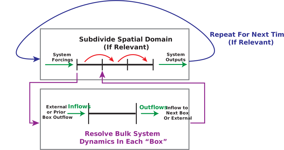
Simulation Model Workflow

Simulation Workflow

Forward Euler, From Taylor Series

Recall \[\frac{df}{dt} = \lim_{\Delta t \to 0}\frac{f(t+\Delta t) - f(t)}{\Delta t}.\]

Pick a small but finite \(\Delta t\) and use the ratio as an approximation.

\[f(t + \Delta t) = f(t) + \Delta t\, f'(t) + \cancel{\color{red}{\frac{\Delta t^2}{2}f''(\xi)} + \text{H.O.T.}}\]

Forward Euler Is First Order

Rearranged, one step:

\[\bbox[5pt, border: 3px solid red]{C(t + \Delta t) = C(t) + \Delta t \cdot g(C(t))}\]

• Local error (per step) is \(\approx O(\Delta t^2)\).
• We take \(T/\Delta t\) steps, so the global error is \(\approx (T/\Delta t) \times \Delta t^2 = O(\Delta t)\).
• Practically: halve \(\Delta t\), halve the error.

Backward Euler

Backward (implicit)

\[C(t+\Delta t) = C(t) + \Delta t\, g(C(t+\Delta t))\]

Evaluate \(g\) at the state you don’t know yet. \(C(t+\Delta t)\) appears on both sides — solving for it is a root-finding problem, the same kind Roots.jl solved for the lake’s thresholds earlier today.

Backward Euler is not more accurate: but it stays better behaved at step sizes that make forward Euler misbehave.

Application: Box Model For An Airshed

What Is A Box Model?

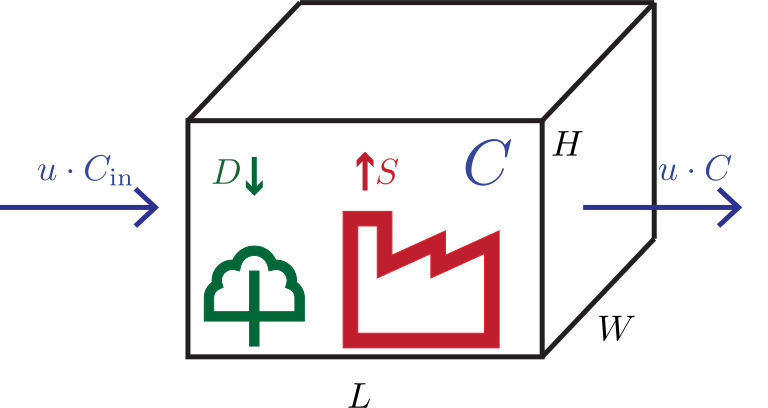
Box models are a common building block of simulation models.

Box models are all about mass-balance (mass \(m\)), often assume well-mixing within the box’s domain.

Can be steady-state \((\dot{m} = 0)\) or not.

Steady-State Box Example

Airshed Model

Variable	Meaning	Units
\(m\)	mass of some air pollutant	g
\(C\)	concentration in box	g/m\(^3\)
\(S, D\)	source, deposition rate within the box	g/s
\(u\)	wind speed	m/s
\(L, W, H\)	box dimensions	m

Selecting Box Dimensions

What is relevant for the box dimensions \(L\), \(W\), and \(H\)?

Primarily the assumption(s) about mixing:

• Mixing height: is there an atmospheric inversion which limits mixing height?
• Homogeneity of input/output flows and emissions.

Steady State

Steady-state box \(\Rightarrow \dot{m} = 0\).

\[\begin{aligned} 0 &= (uWH)C_\text{in} - (uWH)C + S - D \\[0.5em] \Longrightarrow \ C &= C_\text{in} + \frac{S-D}{uWH} \end{aligned}\]

Non-Steady State Model

Now let’s assume some process affecting \(m\) depends on time.

For example: let’s say we care about an air pollutant which has a first-order decay rate \(k\), so \(D(t) = D_0 + km(t)\).

\[ \Rightarrow \frac{dm}{dt} = m_\text{in} - m_\text{out} + S - D_0 - km \]

\[ \dot{m} = \frac{d(CV)}{dt} = \overbrace{(u WH) C_\text{in}}^{\text{inflow}} - \overbrace{(u WH) C}^{\text{outflow}} + \overbrace{S - D_0}^{\text{net emissions}} - \overbrace{kCV}^{\text{mass decay}} \]

Non-Steady State Solution

Solution (derivation here): \(C(t) = \color{red}C_0 e^{-lt} \color{black}+ \color{blue}\frac{P}{l}\left(1 - e^{-lt}\right)\)

• Initial condition is transient (decays to zero eventually);
• Concentration converges to a steady-state solution: ratio of inflows \(P\) and outflows \(l\).

Discretizing the Airshed Model

\[\frac{dC}{dt} = \underbrace{\frac{u}{L} C_\text{in} + \frac{S-D}{V}}_{\Large =P} - \underbrace{\left(\frac{u}{L} + k\right)}_{\Large =l} C\]

\[\frac{C(t+\Delta t) - C(t)}{\Delta t} = P - lC(t)\]

\[\bbox[5pt, border: 3px solid red]{C(t+\Delta t) = C(t) + \Delta t\left(P - lC(t)\right)}\]

Simulation Code

# Raw constants live inside `let` so only the bundle itself becomes global
# Global constants slow down Julia code and are against the style guides --- not critical here, but can matter for "production" code
airshed_params = let
    u, L, W, H = 2.0, 4.0, 4.0, 4.0     # wind speed [m/s], box dimensions [m]
    k = 0.3                             # first-order decay rate       [1/s]
    Ci = 0.2                            # upwind inflow concentration  [g/m³]
    S, D = 10.0, 13.0                   # source, deposition rates     [g/s]
    V = W * H * L

    # The whole model collapses to two numbers: a source strength and a loss rate.
    Psrc = (u / L) * Ci + (S - D) / V   # net source  [g/(m³⋅s)]
    lrate = (u / L) + k                 # total loss rate  [1/s]
    (; u, L, W, H, k, Ci, S, D, V, Psrc, lrate)
end

C0 = 0.1   # initial concentration [g/m³] -- a scenario choice, not a model constant

airshed_rate(C, params) = params.Psrc - params.lrate * C

function airshed_simulate(C_ic, T, Δt, params)
    # round() rather than a bare Int(): Int(10/0.3) throws, and you will
    # eventually pick a Δt that does not divide T exactly.
    steps = Int(round(T / Δt))
    C = zeros(steps + 1)      # index 1 holds the initial condition
    C[1] = C_ic
    for t in 1:steps
        C[t+1] = C[t] + Δt * airshed_rate(C[t], params)
    end
    return C
end

Exact vs. Simulated

T = 10.0
airshed_exact(t, C_ic, params) = C_ic * exp(-params.lrate * t) +
    (params.Psrc / params.lrate) * (1 - exp(-params.lrate * t))

# Starts empty and rises to steady state, rather than decaying to it --- a
# different (and more interesting) transient than "Non-Steady State Solution"
# already showed, using the same equation.
C_empty = 0.0

p_air = plot(xlabel="Time  [s]", ylabel="C  [g/m³]", legend=:topright, xlims=(0, 6))
plot!(p_air, 0:0.01:T, airshed_exact.(0:0.01:T, C_empty, Ref(airshed_params)), color=:black,
    linewidth=5, label="exact")
for (Δt, col) in zip([1.0, 0.5, 0.25], [cb_vermillion, cb_orange, cb_blue])
    plot!(p_air, 0:Δt:T, airshed_simulate(C_empty, T, Δt, airshed_params), color=col, linewidth=3,
        linestyle=:dash, markershape=:circle, markersize=4,
        label="Δt = $Δt")
end
plot!(p_air, size=(1100, 450), left_margin=12mm, right_margin=8mm,
    bottom_margin=12mm, top_margin=5mm)

Figure 3: Forward Euler against the exact solution, for three step sizes.

How Small Should \(\Delta t\) Be?

Every process in your model has a characteristic timescale, \(1/|\text{rate}|\):

System	fastest rate	timescale
Airshed	\(l = 0.8\ \text{s}^{-1}\)	\(1.25\ \text{s}\)
Shallow lake	\(|g| = 0.7\ \text{yr}^{-1}\)	\(1.4\ \text{yr}\)
Climate model	\(|g_{IA}+g_{out}| \approx 0.04\ \text{yr}^{-1}\)	\(24\ \text{yr}\)

\(\Delta t\) must be well inside the shortest timescale in the system.

A Model Actually Worth Simulating

So far the inputs were constant, so the lake settled to a steady state and every \(\Delta t\) agreed. Real airsheds do not sit still.

Let the wind fluctuate, and let there be an emissions episode — a morning traffic peak, a flare, a fire:

Dynamic Simulation Code

# Inputs are functions of TIME, not of step number. 
wind(t) = 2.0 * (1 + 0.4 * sin(2π * t / 60.0))           # wind drifting on a ~1 min cadence [m/s]
emissions(t) = 10.0 + 70.0 * exp(-((t - 6.0) / 1.2)^2)   # episode centered at t = 6 s [g/s]

airshed_rate_dyn(C, t, params) = (wind(t) / params.L) * (params.Ci - C) +
    (emissions(t) - params.D) / params.V - params.k * C

function airshed_dyn(C_ic, T, Δt, params)
    steps = Int(round(T / Δt))
    C = zeros(steps + 1)
    C[1] = C_ic
    for i in 1:steps
        C[i+1] = C[i] + Δt * airshed_rate_dyn(C[i], (i - 1) * Δt, params)
    end
    return C
end

The Inputs

t_range = 0:0.01:14

p_wind = plot(t_range, wind.(t_range), xlabel="Time  [s]", ylabel="Wind speed  [m/s]",
    color=cb_blue, linewidth=3, ylims=(0, 3.0))
p_emit = plot(t_range, emissions.(t_range), xlabel="Time  [s]", ylabel="Emissions  [g/s]",
    color=cb_vermillion, linewidth=3, ylims=(0, 85))
plot(p_wind, p_emit, layout=(1, 2), size=(1100, 450), left_margin=12mm, right_margin=8mm,
    bottom_margin=12mm, top_margin=5mm)

Figure 4: The fluctuating wind and the emissions episode, as functions of time.

The Episode

Td = 20.0
p_ep = plot(xlabel="Time  [s]", ylabel="C  [g/m³]", legend=:topright, xlims=(0, 14))
plot!(p_ep, 0:0.002:Td, airshed_dyn(C0, Td, 0.002, airshed_params), color=:black,
    linewidth=5, label="reference (Δt = 0.002)")
for (Δt, col) in zip([1.0, 0.5, 0.25], [cb_vermillion, cb_orange, cb_blue])
    plot!(p_ep, 0:Δt:Td, airshed_dyn(C0, Td, Δt, airshed_params), color=col, linewidth=3,
        linestyle=:dash, markershape=:circle, markersize=4, label="Δt = $Δt")
end
hline!(p_ep, [1.0], color=cb_green, linewidth=3, linestyle=:dot,
    label="air quality standard")
plot!(p_ep, size=(1100, 450), left_margin=12mm, right_margin=8mm,
    bottom_margin=12mm, top_margin=5mm)

Figure 5: An emissions episode passing through the airshed, at three step sizes.

Another Risk: Grid Size

Having only samples is a potential downside:

• The largest value in your output array is not the largest value of the solution.
• Similar issue with field sampling.

# Stylized, not a real model -- think a brief release event, a rainfall
# spike, anything that rises and falls faster than you expect to sample it.
baseline, spike_height, t_peak, spike_width = 0.1, 1.0, 5.4, 0.3
C_true(t) = baseline + spike_height * exp(-(t - t_peak)^2 / (2 * spike_width^2))

tgrid = 0:1.0:10
recorded_max, max_idx = findmax(C_true.(tgrid))
recorded_t = tgrid[max_idx]

p_samp = plot(xlabel="Time", ylabel="C", legend=:topleft, ylims=(0, 1.25))
plot!(p_samp, 0:0.01:10, C_true.(0:0.01:10), color=:black, linewidth=3,
    label="the actual solution (peak $(round(baseline + spike_height, digits=2)))")
scatter!(p_samp, tgrid, C_true.(tgrid), markersize=8,
    markercolor=cb_vermillion, label="what we compute")
plot!(p_samp, tgrid, C_true.(tgrid), color=cb_vermillion, linewidth=2,
    linestyle=:dash, label="what the plot draws")
annotate!(p_samp, recorded_t + 0.3, recorded_max - 0.1,
    text("recorded max: $(round(recorded_max, digits=2))", 13, cb_vermillion, :left))
plot!(p_samp, size=(600, 500))

Figure 6: A stylized example: a quantity that spikes briefly between two sample points.

Is \(\Delta t\) Small Enough?

1. Name a scalar quantity of interest. Here: the peak concentration, because that is what the standard regulates.
2. Run at \(\Delta t\). Run again at \(\Delta t/2\).
3. If the quantity barely moves, you are converged. If it moves, halve again.
4. Report what you did and what it changed.

Checking Grid Size

\(\Delta t\) [s]	steps	peak \(C\) [g/m³]	change on halving
\(1.0\)	20	\(1.223\)	—
\(0.5\)	40	\(1.025\)	\(16.1\%\)
\(0.25\)	80	\(0.982\)	\(4.2\%\)
\(0.125\)	160	\(0.960\)	\(2.3\%\)
\(0.0625\)	320	\(0.950\)	\(1.0\%\)
\(0.03125\)	640	\(0.945\)	\(0.5\%\)

True peak: \(0.941\). At \(\Delta t = 1\) we are 30% high.

Was Our Error Estimate Correct?

Δts = [1.0, 0.5, 0.25, 0.125, 0.0625, 0.03125]
peak_ref = maximum(airshed_dyn(C0, Td, 0.0005, airshed_params))
errs = [abs(maximum(airshed_dyn(C0, Td, Δt, airshed_params)) - peak_ref) for Δt in Δts]
orders = [round(log2(errs[i] / errs[i+1]), digits=2) for i in 1:length(errs)-1]

p_conv = plot(Δts, errs, xscale=:log10, yscale=:log10, markershape=:circle,
    markersize=7, color=cb_vermillion, linewidth=3, label="forward Euler",
    xlabel="Δt  [s]", ylabel="error in peak  [g/m³]", legend=:bottomright)
# Reference line of slope 1: if our errors run parallel to it, the method is 1st order.
plot!(p_conv, Δts, errs[1] .* (Δts ./ Δts[1]), color=:black, linewidth=2,
    linestyle=:dash, label="slope 1")
plot!(p_conv, size=(1000, 430), left_margin=12mm, right_margin=8mm,
    bottom_margin=12mm, top_margin=5mm)

Figure 7: Error in the peak concentration against step size, on log-log axes.

Observed orders between successive refinements: 1.73, 1.03, 1.13, 1.03, 1.03.

Reading a Log-Log Plot

If \(\text{error} \approx A \Delta t^p\), then

\[\log(\text{error}) = \log A + p \log(\Delta t).\]

• A straight line on log-log axes means the error is a power of \(\Delta t\).
• The slope is that power — the order of the method.
• Slope 1 confirms what Taylor predicted. If you measured slope 0, refining is doing nothing and something else is wrong.

Inputs Must Not Depend on \(\Delta t\)

The scenario itself can’t change when you refine the step size — even a genuinely random one:

Wrong

Random.seed!(1)
steps = Int(T / Δt)
wind_noise = 0.4randn(steps)
wind(i) = 2.0 + wind_noise[i]

Right

Random.seed!(1)
Δt_ref = 0.01  # finer than any Δt we'll use
noise = 0.4randn(Int(T/Δt_ref) + 1)
wind(t) = 2.0 + noise[Int(round(t/Δt_ref))+1]

Key Takeaways

Key Takeaways

• A numerical solution involves computing estimates on a grid.
• Forward Euler is \(C_{t+1} = C_t + \Delta t f(C_t)\), and it is first order: halve \(\Delta t\), halve the error.
• Justify a step size with two steps: the characteristic timescale \(1/|\text{rate}|\) tells you where to start; halving until a named quantity stops moving tells you when to stop.
• On log-log axes, the slope of error against \(\Delta t\) is the error order

Upcoming Schedule

Next Classes

Wednesday: Application to Dissolved Oxygen (Streeter-Phelps)

Next Week: Monte Carlo

Assessments

HW2: Due this Thursday.

HW3: Assigned this week, due Thursday, September 24.

Lab 1: Monday!

Appendix

Non-Steady State Model Solution

\[\begin{aligned} \dot{m} = \frac{d(CV)}{dt} &= \overbrace{(u WH) C_\text{in}}^{\text{inflow}} - \overbrace{(u WH) C}^{\text{outflow}} \\ &\quad + \overbrace{S - D}^{\text{net emissions}} - \overbrace{kCV}^{\text{mass decay}} \\[0.5em] \text{Dividing by } V = WHL\text{:}& \\ \frac{dC}{dt} &= \underbrace{\frac{u}{L} C_\text{in} + \frac{S - D}{V}}_{\Large =P} - \underbrace{\left(\frac{u}{L} + k\right)}_{\Large =l} C \end{aligned}\]

Non-Steady State Model Solution

\[\begin{aligned} \int \frac{dC}{P-lC} &= \int dt \\[0.5em] -\frac{1}{l} \ln\left(P-lC\right) &= t + A \\[0.5em] \underbrace{C(0) = C_0}_\text{initial condition} &\Rightarrow A = -\frac{1}{l} \ln\left(P-lC_0\right) \end{aligned}\]

Non-Steady State Solution

\[\begin{aligned} -\frac{1}{l} \ln\left(\frac{P-lC}{P-lC_0}\right) &= t \\[0.5em] C(t) &= C_0 e^{-lt} + \frac{P}{l}\left(1 - e^{-lt}\right) \end{aligned}\]

References

References