Bifurcations and Hysteresis


Lecture 05

September 9, 2026

Review of Last Class

Feedback Gain

The feedback gain \(g\) measures how strongly a change in the state feeds back on itself.

If \(x = F[p(x, \ldots)]\), then \[g = \frac{\partial F}{\partial x} = \frac{\partial F}{\partial p}\frac{\partial p}{\partial x}.\]

Meanings Of Different Gains

  • \(0 < g < 1\): amplifying but total effect converges to a finite value
  • \(g \geq 1\): amplifying but total effect diverges – will runaway until hitting some other limit
  • \(g < 0\): dampening

With several feedback processes acting at once, the gains add: \[g = \sum_i g_i\]

Equilibria and Stability

An equilibrium \(\hat{X}\) is a state the system stays in:

For \(X_{t+1} = F(X_t)\): \(F(\hat{X}) = \hat{X}\).

  • stable if \(|F'(\hat{X})| < 1\)
  • unstable if \(|F'(\hat{X})| > 1\)

For \(dX/dt = f(X_t)\): \(f(\hat{X}) = 0\).

  • stable if \(|f'(\hat{X})| < 0\)
  • unstable if \(|f'(\hat{X})| > 0\)

The Shallow Lake Problem

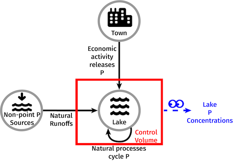
Lake Eutrophication

  • Model introduced by Carpenter et al. (1999).
  • This lecture builds off Quinn et al. (2017).
  • Tradeoff between economic benefits and the health of the lake.

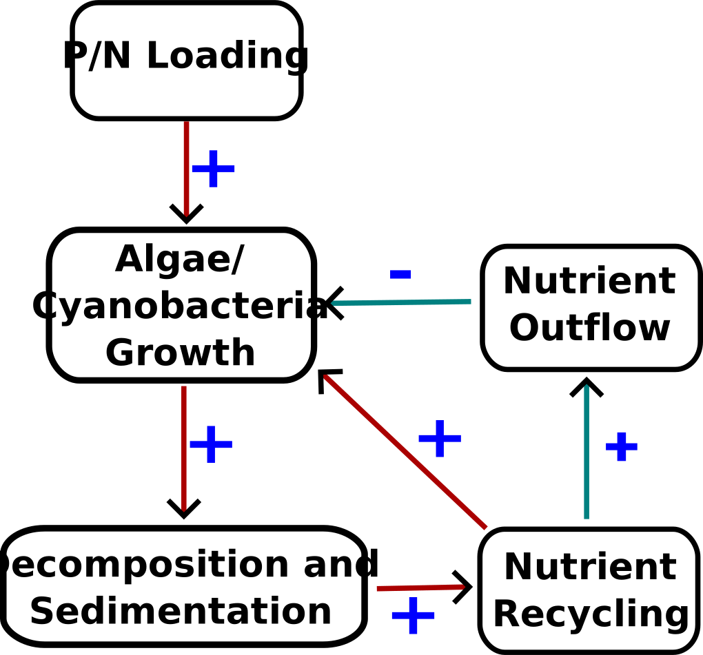
Lake Eutrophication Example

Competition Between Two Feedbacks

Amplifying (sediment recycling):

More P ⇒ More algal biomass ⇒ Reduced O2 ⇒ More Sediment Recycling ⇒ More P

Dampening (loss):

More P ⇒ More outflow and permanent burial ⇒ Less P

Amplifying Feedback Example

The Model

\[P_{t+1} = P_t + \underbrace{L}_{\substack{\text{external} \\ \text{loading}}} - \underbrace{sP_t}_{\substack{\text{outflow +} \\ \text{burial}}} + \underbrace{R(P_t)}_{\substack{\text{sediment} \\ \text{release}}}, \qquad R(P) = r\,\frac{P^q}{m^q + P^q}\]

Variable Meaning Units
\(P_t\) P concentration in the water column at time \(t\) \(\mu\text{g}/\text{L}\)
\(L\) External P loading from the catchment \(\mu\text{g}/(\text{L}\cdot\text{yr})\)

Lake Dynamics Parameters

Parameter Meaning Value
\(s\) removal rate \(0.6\ \text{yr}^{-1}\)
\(r\) maximum sediment release rate \(20\ \mu\text{g}/(\text{L}\cdot\text{yr})\)
\(m\) P concentration at half-maximum release \(30\ \mu\text{g}/\text{L}\)
\(q\) steepness of the sediment release response \(8\)

The Recycling Curve

Code
s = 0.6     # outflow + permanent burial               [1/yr]
r = 20.0    # maximum sediment release rate            [μg/(L⋅yr)]
m = 30.0    # P concentration at half-maximum release  [μg/L]
q = 8       # steepness of the sediment release        [-]

# Fraction of the maximum release rate that is active at concentration P.
# Written as x/(1+x) with x = (P/m)^q: computing P^q and m^q separately
# overflows once q gets large.
recycling_fraction(P, q) = (P / m)^q / (1 + (P / m)^q);

lake_P_release(P, q) = r * recycling_fraction(P, q);
lake_P_loss(P) = s * P;

# One year of lake dynamics.
lake_P_change(P, L, q) = L - lake_P_loss(P) + lake_P_release(P, q);

P_grid = 0:0.1:60

# HW 2's piecewise-linear release: nothing below 25, ramping to the maximum at 35.
R_hw2(P) = P <= 25 ? 0.0 : (P >= 35 ? 20.0 : 20 * (P - 25) / 10)

p_rec = plot(xlims=(0, 60), ylims=(0, 23), legend=:topleft,
    xticks=[0, 10, 20, 25, 35, 40, 50, 60],
    xlabel="P  [μg/L]", ylabel="Sediment release  [μg/(L⋅yr)]")

# Shade the three regimes FIRST so they sit behind the curves.
plot!(p_rec, [0, 25], [0, 0], fillrange=[23, 23], color=cb_blue,
    alpha=0.12, linewidth=0, label=nothing)
plot!(p_rec, [25, 35], [0, 0], fillrange=[23, 23], color=cb_yellow,
    alpha=0.18, linewidth=0, label=nothing)
plot!(p_rec, [35, 60], [0, 0], fillrange=[23, 23], color=cb_vermillion,
    alpha=0.12, linewidth=0, label=nothing)

# Mark the regime boundaries with lines as well as fill -- washed-out colours
# on a projector should not be the only thing separating the three regimes.
for boundary in (25, 35)
    plot!(p_rec, [boundary, boundary], [0, 23], color=:black, linewidth=2,
        linestyle=:dash, label=nothing)
end

plot!(p_rec, P_grid, lake_P_release.(P_grid, q), color=:black, linewidth=5, label="smooth, q = 8")
plot!(p_rec, P_grid, lake_P_release.(P_grid, 12), color=cb_purple, linewidth=3,
    linestyle=:dot, label="smooth, q = 12")
plot!(p_rec, P_grid, R_hw2.(P_grid), color=cb_orange, linewidth=3,
    linestyle=:dash, label="HW 2, piecewise")

annotate!(p_rec, 12, 9, text("oxic:\nsediment holds P", 18, :center))
annotate!(p_rec, 30, 21, text("transition", 18, :center))
annotate!(p_rec, 47.5, 7, text("anoxic:\nreleasing at capacity", 18, :center))
plot!(p_rec, size=(1200, 500), left_margin=10mm)
0 10 20 25 35 40 50 60 P [μg/L] 0 5 10 15 20 Sediment release [μg/(L⋅yr)] smooth, q = 8 smooth, q = 12 HW 2, piecewise
Figure 1: Sediment P release as a function of the lake’s P concentration.

Equilibria and Thresholds

P Sources and Sinks

Code
Pg = 0:0.2:60
L0 = 8.0

# Left panel: where do the sources and sinks cross?
p1_flux = plot(Pg, L0 .+ lake_P_release.(Pg, q), color=:black, linewidth=5,
    label="sources: L + R(P)", legend=:topleft, palette=:tol_muted,
    xlabel="P  [μg/L]", ylabel="Flux  [μg/(L⋅yr)]", ylims=(0, 36))
plot!(p1_flux, Pg, s .* Pg, color=cb_blue, linewidth=3, linestyle=:dash,
    label="sinks: sP")

# Right panel: the net flux, i.e. which way P moves.
net = lake_P_change.(Pg, L0, q)
p2_flux = plot(legend=:topright, framestyle=:zerolines,
    xlabel="P  [μg/L]", ylabel="ΔP  [μg/(L⋅yr)]")
plot!(p2_flux, Pg, zeros(length(Pg)), fillrange=max.(net, 0),
    color=cb_vermillion, alpha=0.20, linewidth=0, label="P rising")
plot!(p2_flux, Pg, min.(net, 0), fillrange=zeros(length(Pg)),
    color=cb_blue, alpha=0.20, linewidth=0, label="P falling")
plot!(p2_flux, Pg, net, color=:black, linewidth=5, label=nothing)

# The only way we know to find the equilibria so far is to solve ΔP = 0 for
# P -- and there are three roots, so we need three starting guesses.
lake_equilibria(L, q) = [Roots.find_zero(P -> lake_P_change(P, L, q), P_guess)
                         for P_guess in [5.0, 30.0, 55.0]];
P_eq = lake_equilibria(L0, q)

# Arrows showing which way the lake moves, generated from the model rather
# than placed by hand. Each arrow is drawn strictly inside the interval it
# belongs to, so no arrow ever points across an equilibrium.
edges = [0.0; P_eq; 60.0]
tails, lengths = Float64[], Float64[]
for i in 1:(length(edges) - 1)
    lo, hi = edges[i], edges[i+1]
    direction = sign(lake_P_change((lo + hi) / 2, L0, q))
    arrow = min(3.0, 0.22 * (hi - lo))
    for centre in (lo + (hi - lo) / 3, hi - (hi - lo) / 3)
        push!(tails, centre - direction * arrow / 2)
        push!(lengths, direction * arrow)
    end
end
quiver!(p2_flux, tails, zeros(length(tails)),
    quiver=(lengths, zeros(length(lengths))), color=:black, linewidth=2)

# NOTE: plot(p1, p2, ...) *copies* the panels, so mutating p1_flux later will
# not update a saved combined figure. Rebuild it with this helper each time.
show_flux() = plot(p1_flux, p2_flux, layout=(1, 2), size=(1150, 480),
    left_margin=12mm, right_margin=8mm, bottom_margin=12mm, top_margin=5mm)
show_flux()
0 10 20 30 40 50 60 P [μg/L] 0 10 20 30 Flux [μg/(L⋅yr)] sources: L + R(P) sinks: sP 0 10 20 30 40 50 60 P [μg/L] −6 −3 0 3 6 ΔP [μg/(L⋅yr)] P rising P falling
Figure 2: P sources and sinks at a loading of 8 μg/(L·yr), and the resulting net flux.

Three Equilibria

Code
scatter!(p1_flux, P_eq, s .* P_eq, markersize=9, markercolor=cb_orange,
    label="equilibria")
scatter!(p2_flux, P_eq, zeros(length(P_eq)), markersize=9,
    markercolor=cb_orange, label=nothing)
show_flux()
0 10 20 30 40 50 60 P [μg/L] 0 10 20 30 Flux [μg/(L⋅yr)] sources: L + R(P) sinks: sP equilibria 0 10 20 30 40 50 60 P [μg/L] −6 −3 0 3 6 ΔP [μg/(L⋅yr)] P rising P falling
Figure 3: The three equilibria at a loading of 8 μg/(L·yr).

Stability, Formally

\[\begin{gathered} F'(P) = 1 + \underbrace{R'(P)}_{\substack{\text{amplifying} \\ \text{(sediment)}}} - \underbrace{s}_{\substack{\text{dampening} \\ \text{(loss)}}} = 1 + g(P) \\ R'(P) = \frac{rq}{P}\frac{x}{(1+x)^2},\ x = \left(\frac{P}{m}\right)^q \end{gathered}\]

Stablity requires \(|F'| < 1\), or: \[\bbox[5pt, border: 3px solid red]{g(P) < 0 \quad \Longleftrightarrow \quad R'(P) < s}\]

Gain at the Three Equilibria

Code
# Slope of the recycling curve: the strength of the amplifying loop.
release_slope(P, q) = r * q * (P / m)^q / (P * (1 + (P / m)^q)^2);

# Feedback gain: amplifying (sediment) minus dampening (loss).
feedback_gain(P, q) = release_slope(P, q) - s;
\(\hat{P}\) \(g = R'(\hat{P}) - s\) \(F' = 1 + g\)
\(13.4\) \(-0.6\) \(0.4\) stable (oligotrophic)
\(30.0\) \(+0.7\) \(1.7\) unstable
\(45.5\) \(-0.5\) \(0.5\) stable (eutrophic)

The unstable equilibrium is a mathematical artifact: no lake is ever found in it.

What Happens As \(L\) Changes?

Code
# L only shifts the sources curve up and down -- the sinks line never moves.
# The middle curve is the L = 8 one we have been using all along; redraw it so
# the legend names its loading alongside the other two. It lands exactly on
# top of the black curve already there.
plot!(p1_flux, Pg, 2.0 .+ lake_P_release.(Pg, q), color=cb_green, linewidth=3, label="L = 2")
plot!(p1_flux, Pg, 8.0 .+ lake_P_release.(Pg, q), color=:black, linewidth=3, label="L = 8")
plot!(p1_flux, Pg, 12.0 .+ lake_P_release.(Pg, q), color=cb_vermillion, linewidth=3, label="L = 12")
plot!(p1_flux, legend=:topleft, ylims=(0, 36))
plot!(p1_flux, size=(1200, 500), left_margin=10mm)
0 10 20 30 40 50 60 P [μg/L] 0 10 20 30 Flux [μg/(L⋅yr)] sources: L + R(P) sinks: sP equilibria L = 2 L = 8 L = 12
Figure 4: Raising the external loading shifts the sources curve up rigidly.

What Happens at the Threshold

Somewhere between \(L = 8\) and \(L = 12\), two equilibria collide and annihilate.

At that loading the sources curve is tangent to the sinks line — same value and same slope:

\[R'(P) = s \qquad \Longleftrightarrow \qquad g(P) = 0 \qquad \Longleftrightarrow \qquad F'(P) = 1\]

This is a bifurcation: as the loading crosses a threshold, the number and/or stability of equilibria changes.

Finding Equilibria as \(L\) Changes

This raises the question:

Which values of \(P\) are equilibria, for a given \(L\)?

Why Is This Hard?

\[L - s\hat{P} + r\frac{\hat{P}^q}{m^q + \hat{P}^q} = 0\]

  • \(\hat{P}\) is buried inside a degree-\(q\) nonlinearity, so there is no closed form.
  • There are up to three roots — but this varies based on \(L\) and not predictably.

Solve for \(L\), Not \(P\)

Turn the question around:

Which value of \(L\) makes a given \(P\) an equilibrium?

Same equation, but now \(L\) sits alone: \[\bbox[5pt, border: 3px solid red]{L(P) = sP - R(P)}\]

Bifurcation Diagram

Code
# Solve for L as a function of P
loading_for_P(P, q) = lake_P_loss(P) - lake_P_release(P, q);


Pb = 0.01:0.02:60.0
L_eq = loading_for_P.(Pb, q)

# Both thresholds sit where the recycling curve and the loss line have the
# same slope, so the feedback gain is zero. Below m the lake eutrophies;
# above m it can recover.
eutrophic_P(q) = Roots.find_zero(P -> feedback_gain(P, q), (0.1, m));
recovery_P(q) = Roots.find_zero(P -> feedback_gain(P, q), (m, 80.0));
eutrophication_threshold(q) = loading_for_P(eutrophic_P(q), q);
recovery_threshold(q) = loading_for_P(recovery_P(q), q);

# Split the curve into stable and unstable branches. Mask with NaN rather than
# indexing: NaN breaks the line, whereas indexing would draw a spurious
# horizontal segment straight across the bistable window.
is_stable = feedback_gain.(Pb, q) .< 0
L_st = [st ? Lv : NaN for (Lv, st) in zip(L_eq, is_stable)]
L_un = [st ? NaN : Lv for (Lv, st) in zip(L_eq, is_stable)]

L_eutrophic, P_eutrophic = eutrophication_threshold(q), eutrophic_P(q)
L_recover, P_recover = recovery_threshold(q), recovery_P(q)

# Legend goes bottom-right: the top-left corner is where the upper stable
# branch lives, and an opaque legend box there would hide it.
p_bif = plot(xlims=(0, 20), ylims=(0, 60), legend=:bottomright, palette=:tol_muted,
    xlabel="External loading L  [μg/(L⋅yr)]", ylabel="Equilibrium P  [μg/L]")
# Shade the bistable window first so it sits behind the curves.
plot!(p_bif, [L_recover, L_eutrophic], [0, 0], fillrange=[60, 60], color=:grey,
    alpha=0.18, linewidth=0, label="bistable window")
plot!(p_bif, L_st, Pb, color=:black, linewidth=5, label="stable")
plot!(p_bif, L_un, Pb, color=:black, linewidth=3, linestyle=:dash, label="unstable")
scatter!(p_bif, [L_eutrophic, L_recover], [P_eutrophic, P_recover], markersize=10,
    markercolor=cb_vermillion, label="thresholds")

annotate!(p_bif, L_eutrophic + 0.5, P_eutrophic + 8,
    text("eutrophication\nL = $(round(L_eutrophic, digits=1))", 15, :left))
annotate!(p_bif, L_recover - 0.5, P_recover + 5,
    text("recovery\nL = $(round(L_recover, digits=1))", 15, :right))
plot!(p_bif, size=(1150, 500), left_margin=12mm, right_margin=8mm, bottom_margin=12mm, top_margin=5mm)
0 5 10 15 20 External loading L [μg/(L⋅yr)] 0 10 20 30 40 50 60 Equilibrium P [μg/L] bistable window stable unstable thresholds
Figure 5: Equilibrium P as a function of external loading, with both thresholds marked.

Reading the Bifurcation Diagram

  • Below \(L = 5.3\): only the oligotrophic state exists.
  • Above \(L = 11.7\): only the eutrophic state exists.
  • In between: both, separated by the dashed boundary.

Hysteresis

What Is Required To Restore A Lake?

Suppose loading crept up to \(L = 13\) and the lake became eutrophic.

We reduce loading to \(L = 11\) — below the threshold that broke it.

Does the lake recover?

Hysteresis

Code
# Raise L one small step at a time, letting the lake fully relax at each step
# and carrying the final state forward as the next initial condition.
#
# Do NOT use a continuous ramp instead: relaxation time diverges at a threshold, so
# even a very slow ramp fires the transition well past the true threshold. That
# overshoot is real (it is critical slowing down), but it draws a misleading
# picture of *where* the threshold is.
function quasistatic_sweep(Ls, P_ic; tol=1e-9, maxiter=50_000)
    P = P_ic
    out = zeros(length(Ls))
    for (i, L) in enumerate(Ls)
        for _ in 1:maxiter
            Pn = P + lake_P_change(P, L, q)
            converged = abs(Pn - P) < tol
            P = Pn
            converged && break
        end
        out[i] = P
    end
    return out
end

function simulate_lake_P(P_ic, T, L, q)
    P = zeros(T)
    P[1] = P_ic
    for t = 2:T
        P[t] = P[t-1] + lake_P_change(P[t-1], L, q)
    end
    return P
end

L_up = collect(0:0.05:20)
L_dn = reverse(L_up)
P_up = quasistatic_sweep(L_up, 0.0)
P_dn = quasistatic_sweep(L_dn, P_up[end])

p_hyst = plot(xlims=(0, 20), ylims=(0, 60), legend=:topleft,
    xlabel="External loading L  [μg/(L⋅yr)]", ylabel="P  [μg/L]")
plot!(p_hyst, L_eq, Pb, color=:grey, alpha=0.35, linewidth=2, label=nothing)
plot!(p_hyst, L_up, P_up, color=cb_vermillion, linewidth=5, label="loading up")
# Dashed, so you can still see the red path underneath where the two coincide
# -- which is everywhere outside the bistable window. That is the whole point.
plot!(p_hyst, L_dn, P_dn, color=cb_blue, linewidth=4, linestyle=:dash,
    label="loading down")
scatter!(p_hyst, [L_eutrophic, L_recover], [P_eutrophic, P_recover], markersize=8,
    markercolor=:black, label=nothing)
annotate!(p_hyst, L_eutrophic - 0.5, 44, text("eutrophication", 14, :right))
annotate!(p_hyst, L_recover + 0.5, 21, text("recovery", 14, :left))

# Right: same L, two initial conditions either side of the unstable point.
T = 60
p_basin = plot(legend=:right, xlabel="Year", ylabel="P  [μg/L]", ylims=(0, 60))
plot!(p_basin, simulate_lake_P(31.0, T, L0, q), color=cb_vermillion, linewidth=4,
    label=L"P_0 = 31")
plot!(p_basin, simulate_lake_P(30.0, T, L0, q), color=:grey, linewidth=3,
    linestyle=:dot, label=L"P_0 = 30")
plot!(p_basin, simulate_lake_P(29.0, T, L0, q), color=cb_blue, linewidth=4,
    label=L"P_0 = 29")

plot(p_hyst, p_basin, layout=(1, 2), size=(1200, 490),
    left_margin=12mm, right_margin=8mm, bottom_margin=12mm, top_margin=5mm)
0 5 10 15 20 External loading L [μg/(L⋅yr)] 0 10 20 30 40 50 60 P [μg/L] loading up loading down 0 10 20 30 40 50 60 Year 0 10 20 30 40 50 60 P [μg/L]
Figure 6: Left: a quasi-static loading sweep up and back down. Right: two trajectories either side of the unstable equilibrium.

“Memory” Means You Need To Overshoot Cuts To Recover

  • Eutrophication at \(L = 11.7\)
  • Recovery at \(L = 5.3\)

You must cut loading 54% below the level that caused the eutrophication to restore the lake: recovery is more “expensive” than maintanence.

Losing Resilience

How does a oligotrophic lake respond to a one-off P pulse?

\(L\) \(\hat{P}\) \(g\) \(F'\) recovery time (\(0.1\) P)
\(8.0\) \(13.4\) \(-0.6\) \(0.4\) \(6\)
\(10.0\) \(17.0\) \(-0.5\) \(0.5\) \(7\)
\(11.0\) \(19.3\) \(-0.4\) \(0.6\) \(10\)
\(11.5\) \(21.0\) \(-0.2\) \(0.8\) \(20\)
\(11.6\) \(21.5\) \(-0.1\) \(0.9\) \(30\)
\(11.7\) \(22.6\) \(0.0\) \(1.0\) \(\infty\)

Where Did \(r\) Come From?

We treated the maximum recycling rate \(r\) as a constant. But it is really \(\kappa M\), where \(M\) is the sediment P pool — a stock that fills over decades:

\[\begin{aligned} P_{t+1} &= P_t + L - s_\text{out}P_t - hP_t + \kappa M_t\,\frac{P_t^q}{m^q + P_t^q} \\[0.4em] M_{t+1} &= M_t + hP_t - bM_t - \kappa M_t\,\frac{P_t^q}{m^q + P_t^q} \end{aligned}\]

with \(s_\text{out} + h = s\).

Fifty Years of Boring Data

Code
function simulate_two_stock(P_ic, M_ic, T; L=11.5, s_out=0.2, h=0.4, b=0.015, kappa=0.1)
    P, M = zeros(T), zeros(T)
    P[1], M[1] = P_ic, M_ic
    for t in 2:T
        rec = kappa * M[t - 1] * recycling_fraction(P[t-1], q)
        P[t] = P[t - 1] + L - s_out * P[t - 1] - h * P[t - 1] + rec
        M[t] = M[t - 1] + h * P[t - 1] - b * M[t - 1] - rec
    end
    return P, M
end

# The eutrophication threshold when the sediment can supply at most r_eff = kappa*M.
function eutrophication_threshold_at(r_eff)
    Ps = collect(0.01:0.01:m)
    return maximum(lake_P_loss.(Ps) .- r_eff .* recycling_fraction.(Ps, q))
end

L_held = 11.5                      # BELOW the one-stock threshold of 11.7
T2 = 140
P2, M2 = simulate_two_stock(L_held / s, 0.0, T2)
yrs = 0:(T2 - 1)

fonts = (guidefontsize=15, tickfontsize=13, titlefontsize=17, legendfontsize=12)

# The one-stock model's eutrophication threshold, recomputed each year from the
# sediment the lake has actually accumulated.
thr = eutrophication_threshold_at.(0.1 .* M2)
danger = findall(thr .< L_held)      # years with no oligotrophic equilibrium left
flip_yr = findfirst(>(35), P2) - 1

p_mon = plot(yrs, P2, color=:black, linewidth=5, legend=false, ylims=(0, 60),
    xlabel="Year", ylabel="P  [μg/L]", title="What we measure"; fonts...)

p_hid = plot(yrs, M2, color=cb_green, linewidth=5, legend=false,
    xlabel="Year", ylabel="Sediment P, M  [μg/L]",
    title="What we don't"; fonts...)

p_thr = plot(ylims=(10.8, 18.5), legend=:topright, xlabel="Year",
    ylabel="L  [μg/(L⋅yr)]", title="Why it flips"; fonts...)
# Shade the years when the threshold has slid below the loading -- so the
# oligotrophic equilibrium no longer exists, at a loading that never moved.
plot!(p_thr, [yrs[first(danger)], yrs[last(danger)]], [10.8, 10.8],
    fillrange=[18.5, 18.5], color=cb_vermillion, alpha=0.13, linewidth=0, label=nothing)
plot!(p_thr, yrs, thr, color=cb_vermillion, linewidth=5, linestyle=:dash,
    label="eutrophication threshold")
hline!(p_thr, [L_held], color=:black, linewidth=3, label="actual loading")

# Mark the year the lake flipped on all three panels: same instant, three views.
for p in (p_mon, p_hid, p_thr)
    vline!(p, [flip_yr], color=:grey, linestyle=:dot, linewidth=2, label=nothing)
end

plot(p_mon, p_hid, p_thr, layout=(1, 3), size=(1250, 440),
    left_margin=11mm, right_margin=6mm, bottom_margin=12mm, top_margin=5mm)
0 25 50 75 100 125 Year 0 10 20 30 40 50 60 P [μg/L] What we measure 0 25 50 75 100 125 Year 0 50 100 150 200 250 Sediment P, M [μg/L] What we don't 0 25 50 75 100 125 Year 12 14 16 18 L [μg/(L⋅yr)] Why it flips eutrophication threshold actual loading
Figure 7: A lake held at a constant, apparently safe loading of 11.5 μg/(L·yr).

Key Takeaways

Key Takeaways

  • A bifurcation is a change in equilibria: it happens exactly where the amplifying and dampening loops cancel, \(g = 0\) and \(F' = 1\).
  • The unstable equilibrium is a boundary, not a “true” state.
  • Hysteresis: the eutrophication and recovery thresholds are different, so restoring the loading does not restore the lake.
  • Approaching a threshold you lose resilience: recovery slows.

Upcoming Schedule

Next Classes

Monday: Computational Models and Simulation

Assessments

Homework 2: Due next Thursday (September 17) at 9pm.

Reading (5750): Carpenter et al. (1999)

References

References

Carpenter, S. R., Ludwig, D., & Brock, W. A. (1999). Management of eutrophication for lakes subject to potentially irreversible change. Ecol. Appl., 9(3), 751–771. https://doi.org/10.2307/2641327
Quinn, J. D., Reed, P. M., & Keller, K. (2017). Direct policy search for robust multi-objective management of deeply uncertain socio-ecological tipping points. Environmental Modelling & Software, 92, 125–141. https://doi.org/10.1016/j.envsoft.2017.02.017