Stability and Examples

---

Lecture 04

September 2, 2026

Overview

• Review of Last Class
• Stability of Systems
• Example: Simple Climate Model
• Stability Example: Lotka-Volterra
• Key Takeaways
• Upcoming Schedule

Review of Last Class

Feedbacks

Feedback Types

Feedbacks are “loops” in a system diagram.

Feedbacks can be:

• Amplifying (sometimes called “positive”)
• Dampening (sometimes called “negative”)

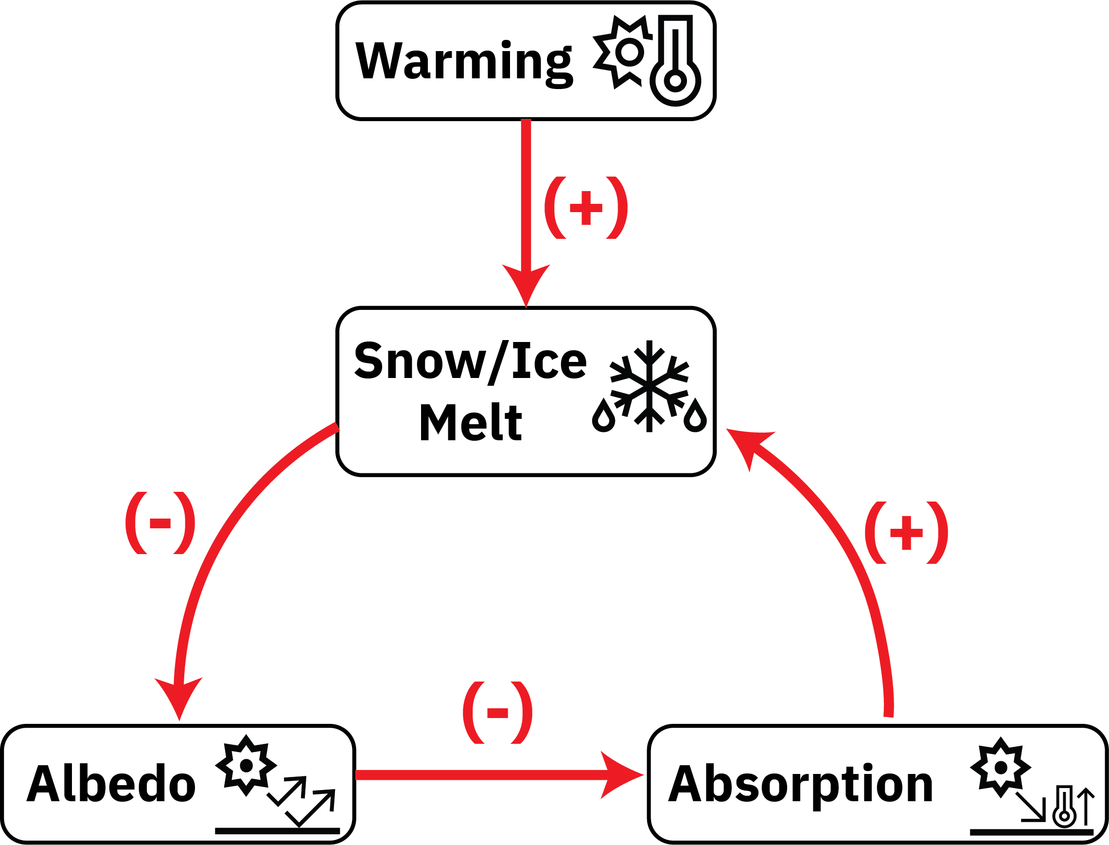
Ice-Albedo Feedback Loop

Feedback Level

With no feedback: \(\text{Total Effect} = \text{Direct Effect}\)

Over one pass feedback loop: \(\text{Total Effect} = (1+g) (\text{Direct Effect})\)

\(g\) is the feedback factor (or gain): \(g > 0\) means amplification, \(g < 0\) means dampening.

Calculating \(g\)

If \(x = F[p(x, \ldots)]\), \[g = \frac{\partial F}{\partial x} = \frac{\partial F}{\partial p} \frac{\partial p}{\partial x}.\]

With multiple feedback processes (\(x = F[p_1(x, \ldots), p_2(x, \ldots), \ldots]\)):

\[g = \sum_i \frac{\partial F}{\partial p_i} \frac{\partial p_i}{\partial x} = \sum_i g_i.\]

Multiple Feedback Passes

\[\begin{aligned} \text{Total Effect} &= (\text{Direct Effect})\left(1 + g + g^2 + g^3 + \ldots\right) \\[0.5em] &= \frac{\text{Direct Effect}}{1-g} \qquad \text{(when $|g| < 1$)} \end{aligned}\]

• if \(0 < g < 1\): amplifying but stable feedback
• if \(g < 0\): dampening feedback
• if \(g > 1\): system instability

Fixed Points (Equilibria)

System dynamics are often understood relative to their equilibria (or fixed points).

• If \(X_{t+1} = F(X_t)\), equilibria occur where \(F(X_t) = X_t\).
• If \(\frac{dx}{dt} = f(x)\), equilibria occur where \(f(x) = 0\).

In other words, a system at an equilibrium will stay at an equilibrium.

Stability of Systems

Single-Equation System

If our model consists of one differential equation, \[\frac{dX}{dt} = F(X)\]
then the equilibria are the solutions to \(F(\hat{X}) = 0\).

Stability to Small Perturbations

Now suppose we perturb the system slightly from an equilibrium \(\hat{X}\) to \(\hat{X} + \Delta X\).

Let \(X(t)\) be the solution with this new initial condition and define \[X(t) = \hat{X} + \Delta X(t).\]

How can we analyze the behavior of the system after this perturbation?

Taylor Approximation

For a small perturbation, we can linearize the system around the equilibrium \(\hat{X}\) using the Taylor approximation \[F(\hat{X} + \Delta X) \approx F(\hat{X}) + \Delta X \left.\frac{\partial F(X)}{\partial X}\right|_{\hat{X}}.\]

Simplifying Taylor Approximation

But then since \(\hat{X}\) is time-independent and \(F(\hat{X}) = 0\):

\[ \frac{d[\Delta X(t)]}{dt} \approx \Delta X \left.\frac{dF(X)}{dX}\right|_{\hat{X}} \]

Implications for Stability

• If \(\frac{dF}{dX} < 0\), then \(\Delta X\) will decay to zero, \(X\) will return to \(\hat{X}\), and the system is stable.
• If \(\frac{dF}{dX} > 0\), then \(\Delta X\) will grow, \(X\) will diverge from \(\hat{X}\), and the system is unstable.

General Model Form

Suppose our model consists of a system of differential equations

\[\begin{aligned} \frac{dX_1}{dt} = F_1(X_1, X_2, \ldots, X_n) \\ \frac{dX_2}{dt} = F_2(X_1, X_2, \ldots, X_n) \\ \vdots \\ \frac{dX_n}{dt} = F_n(X_1, X_2, \ldots, X_n) \end{aligned}\]

Equilibria

The equilibria for this system are the solutions to

\[F_i(\hat{X}_1, \hat{X}_2, \ldots, \hat{X}_n) = 0 \quad \text{for all } i = 1, 2, \ldots, n.\]

Stability to Small Perturbations

Similarly to before, now suppose we perturb the system slightly from an equilibrium \(\hat{X}_i\) to \(\hat{X}_i + \Delta X_i\).

Let \(X_i(t)\) be the solution with this new initial condition and define \[X_i(t) = \hat{X}_i + \Delta X_i(t).\]

Taylor Approximation

Assume that the perturbation \(\Delta X_i(t)\) is “small”. Recall the multivariate Taylor expansion (2d for simplicity):

\[\begin{aligned} f(X_1, X_2) \approx &f(\hat{X}_1, \hat{X}_2) + \Delta X_1 \left.\frac{\partial f(X_1, X_2)}{\partial X_1}\right|_{(\hat{X}_1, \hat{X}_2)} \\ &+ \Delta X_2\left.\frac{\partial f(\hat{X}_1, \hat{X}_2)}{\partial X_2}\right|_{(\hat{X}_1, \hat{X}_2)} \end{aligned}\]

Taylor Approximation For Our System

Then:

\[\begin{aligned} F_i(\hat{X}_1 + &\Delta X_1, \hat{X}_2 + \Delta X_2, \ldots, \hat{X}_n + \Delta X_n) \\ \qquad \approx &F_i(\hat{X}_1, \hat{X}_2, \ldots, \hat{X}_n) \\[0.5em] &+ \sum_{j=1}^n \Delta X_j \left.\frac{\partial F_i(X_1, X_2, \ldots, X_n)}{\partial X_j}\right|_{(\hat{X}_1, \hat{X}_2, \ldots, \hat{X}_n)} \end{aligned}\]

Simplifying Taylor Approximation

But then since \(\hat{X}_i\) are time-independent and \(F_i(\hat{X}_1, \hat{X}_2, \ldots, \hat{X}_n) = 0\):

\[ \frac{d[\Delta X_i(t)]}{dt} \approx \sum_{j=1}^n \Delta X_j \left.\frac{\partial F_i(X_1, X_2, \ldots, X_n)}{\partial X_j}\right|_{(\hat{X}_1, \hat{X}_2, \ldots, \hat{X}_n)} \]

Converting to Matrix Form

Construct a matrix \(A\) (the Jacobian) with elements \[a_{ij} = \left.\frac{\partial F_i(X_1, X_2, \ldots, X_n)}{\partial X_j}\right|_{(\hat{X}_1, \hat{X}_2, \ldots, \hat{X}_n)}\]

and a vector \(\mathbf{\Delta X} = [\Delta X_1, \Delta X_2, \ldots, \Delta X_n]^T\).

Then we can write the system of equations as

\[\frac{d[\mathbf{\Delta X}]}{dt} \approx A \mathbf{\Delta X}\]

Eigenvalues and Stability

The eigenvalues of \(A\) determine the stability of the system:

• If all eigenvalues have negative real parts, the system is stable.
• If any eigenvalue has a positive real part, the system is unstable.
• If any eigenvalue has a zero real part and non-zero imaginary part, the system is degenerate and solutions oscillate around the equilibrium (sometimes called marginally stable).

Stability for Single-Equation System

If we only have one equation, this is simpler:

Stability and Resilience

Can think of stable equilibria as suggesting “resilience”: small disruptions to the system state will fade away with time and the system will stabilize.

Unstable equilibria: small shocks amplify and the system will deviate from its “typical” state.

Generalization to Difference Equations

Suppose instead of a system of ODEs, we have a system of difference equations:

\[X_{i, t+1} = F_i(X_{1, t}, X_{2, t}, \ldots, X_{n, t})\]

Generalization to Difference Equations

Then we also want to look at the Jacobian, but the condition is slightly different:

• The system is stable if all eigenvalues of the Jacobian have magnitude less than 1.
• The system is unstable if any eigenvalue of the Jacobian has magnitude greater than 1.
• The system is degenerate if any eigenvalue of the Jacobian has magnitude equal to 1.

Example: Simple Climate Model

“Snowball Earth” and Ice-Albedo Feedback

In the Neoproterozoic Era (550-1000 million years ago), the Earth was covered by ice and snow during two global glaciation events.

One theory is “Snowball Earth” melted due to a combination of a one-off increase in CO\(_2\) (due to volcanic outgassing) and the ice-albedo feedback.

Simple (Zero-D) Climate Model

A simple climate model (with no sustained CO\(_2\) emissions) with the ice-albedo feedback can be written as

\[C\frac{dT}{dt} = F(T) = \frac{S(1-\alpha)}{4} - (A - BT)\]

Simple Climate Model Terms

\[\frac{dT}{dt} = F(T) = \frac{1}{C}\left(\frac{S(1-\alpha)}{4} - (A - BT)\right)\]

• \(S\approx 1368\ \text{W}/\text{m}^2\): incoming solar insolation,
  
• \(C \approx 5\ \text{J}/\text{m}^2/ ^\circ\text{C}\): heat capacity of the mixed atmosphere and upper ocean,
  
• \(B=-1.3\ \text{W}/\text{m}^2/^\circ\text{C}\): outgoing radiation feedback factor,
• \(A=221.2\ \text{W}/\text{m}^2\): constant for outgoing radiation (based on a stable pre-industrial temperature of 14°C).

Ice-Albedo Feedback

One possible function for \(\alpha(T)\): \[ \alpha(T) = \begin{cases} \alpha_{i} & \mbox{if }\;\; T \leq -10\text{°C}\\ \alpha_{i} + (\alpha_{0}-\alpha_{i})\frac{T + 10}{20} & \mbox{if }\;\; -10\text{°C} \leq T \leq 10\text{°C} \\ \alpha_{0} &\mbox{if }\;\; T \geq 10\text{°C} \end{cases} \]

Can choose \(\alpha_i = 0.5\) and \(\alpha_0 = 0.3\).

Ice-Albedo Feedback Function

function calc_albedo(T; α0=0.3, αi=0.5, ΔT=10)
    if T < -ΔT
        return αi
    elseif -ΔT <= T < ΔT
        return αi + (α0-αi)*(T+ΔT)/(2ΔT)
    elseif T >= ΔT
        return α0
    end
end

T_example = -20:1:20
p = plot([-20, -10], [0.2, 0.2], fillrange=[0.6, 0.6], color=:lightblue, alpha=0.2, label=nothing)
plot!([10, 20], [0.2, 0.2], fillrange=[0.6, 0.6], color=:red, alpha=0.12, label=nothing)
plot!(T_example, calc_albedo.(T_example), lw=3., label="α(T)", color=:black)
plot!(ylabel="albedo α\n(planetary reflectivity)", xlabel="Temperature [°C]")
annotate!(-15.5, 0.252, text("completely\nfrozen", 16, :darkblue))
annotate!(15.5, 0.252, text("no ice", 16, :darkred))
annotate!(-0.3, 0.252, text("partially frozen", 16, :darkgrey))
plot!(size=(1000, 500), ylims=(0.2, 0.6))

Figure 1: Ice-Albedo Feedback Function

Ice-Albedo Feedback Gain

Focus on the range of \(T\) where \(\alpha(T)\) is not constant (i.e., \(-10^\circ\text{C} < T < 10^\circ\text{C}\)).

\[\begin{aligned} g_{IA} &= \frac{\partial F}{\partial \alpha} \frac{d\alpha}{dT} \\ &= \frac{-S}{4C} \cdot \frac{\alpha_0 - \alpha_i}{20} \\ &= \frac{-1368}{4*51} \cdot \frac{0.3 - 0.5}{20} \\ &\approx 0.07 \end{aligned}\]

Outgoing Radiation Feedback

\[g_{out} = \frac{\partial F}{\partial T} = \frac{B}{C} = \frac{-1.3}{51} \approx -0.03\]

So the total feedback is \(g_{total} = g_{IA} + g_{out} \approx 0.04\).

Total Climate Model Feedback

To Sum:

• When \(\alpha\) is constant (\(T < -10^\circ\text{C}\) or \(T > 10^\circ\text{C}\)), the total feedback is negative (impact of a temperature perturbation is dampened by \(1/(1-g_{out}) \approx 0.97\)).
• When \(\alpha\) can vary (\(-10^\circ\text{C} < T < 10^\circ\text{C}\)), the total feedback is positive (a temperature perturbation in this temperature range is amplified by a factor of \(1/(1-g_{total}) \approx 1.04\)).

Equilibria of Model

# constants
S = 1368 # solar insolation W/m^2
C = 51 # heat capacity J/m^2/°C
B = -1.3 # outgoing radiation feedback factor J/m^2/°C
A =  S * (1 - 0.3) / 4 + (B * 14) # J/m^2

T_range = -60:0.1:30
# absorbed solar radiation
ASR(T) = (S * (1- calc_albedo(T))) / 4
IR = ASR.(T_range) # absorbed radiation
# outgoing radiation
OTR(T) = A - B * T
OR = OTR.(T_range) # outgoing radiation
imbalance = IR - OR

p1_stability = plot(legend=:topleft, ylabel="Energy Flux (W/m²)", xlabel="Temperature (°C)")
plot!(p1_stability, T_range, OR, label="Outgoing Radiation", color=:blue, lw=3)
plot!(p1_stability, T_range, IR, label="Absorbed Radiation", color=:orange, lw=3)

p2_stability = plot(ylims=(-50, 45), ylabel="Energy Flux (W/m²)", xlabel="Temperature (°C)")
plot!([-60, 30], [-100, -100], fillrange=[0, 0], color=:blue, alpha=0.1, label=nothing)
plot!([-60, 30], [100, 100], fillrange=[0, 0], color=:red, alpha=0.1, label=nothing)
annotate!(-58, -40, text("cooling", :left, :darkblue))
annotate!(-58, 38, text("warming", :left, :darkred))
plot!(p2_stability, T_range, imbalance, label="Radiative Imbalance", color=:black, lw=3)
p_stability = plot(p1_stability, p2_stability, layout=(1, 2), size=(1100, 500), left_margin=5mm)

Figure 2: Ice-Albedo Feedback Function

Finding Equilibria

One is easy: we designed the model to have an equilibrium at \(T = 14^\circ\text{C}\) (how we solved for \(A\)).

Let’s find the others numerically using Roots.jl:

F(T) = (1 / C) * (ASR(T) - OTR(T))
T₁ = Roots.find_zero(F, 0)
T₂ = Roots.find_zero(F, -40)
@show (T₁, T₂);

(T₁, T₂) = (7.547169811320748, -38.61538461538461)

Equilbiria of Ice-Albedo Model

There are three equilibria for this model:

• \(T = 14^\circ\text{C}\) (pre-industrial warm climate)
• \(T = 7.55^\circ\text{C}\) (alternative unstable climate)
• \(T = -38.6^\circ\text{C}\) (alternative frozen climate)

Stability of Ice-Albedo Model

We computed the relevant derivatives when computing the gain of the feedbacks:

• At \(T = 14^\circ\text{C}\) and \(T = -38.6^\circ\text{C}\), \(\frac{\partial F}{\partial T} = -0.03\), so these equilibria are stable.
• At \(T = 7.55^\circ\text{C}\), \(\frac{\partial F}{\partial T} = 0.04\), so this equilibrium is unstable.

Numerical Simulation of Stability

function energy_balance_model(T₀, CO₂; B = -1.3)
    S = 1368 # solar insolation W/m^2
    C = 51 # heat capacity 
    A =  S * (1 - 0.3) / 4 + (B * 14)
    Δt = 1 # annual time step
    CO₂_preindustrial = 280.0
    F = 5.0 * log.(CO₂ / CO₂_preindustrial)
    L = length(CO₂)
    T = zeros(L)
    T[1] = T₀
    for t = 1:L-1
        α = calc_albedo(T[t])
        rad_in = S * (1 - α) / 4 # absorbed solar radiation
        T[t+1] = T[t] + ((rad_in) - (A - B * T[t]) + F[t]) / C * Δt 
    end
    return T
end

initial_T = -60:5:40
T = map(s -> energy_balance_model(s, 280ones(200)), initial_T)
p = plot(T, label=:false)
plot!(energy_balance_model(7.547, 280ones(200)), color=:grey, label=:false, legend=:outerright, left_margin=5mm, bottom_margin=10mm)
scatter!([200], [14], color=:orange, markershape=:circle, markersize=8, label="Pre-Industrial Warm Climate")
scatter!([200], [7.547], color=:grey, markershape=:circle, markersize=8, label="Alternative Unstable Climate")
scatter!([200], [-38.6], color=:blue, markershape=:circle, markersize=8, label="Alternative Frozen Climate")
xlims!(0, 205)
yticks!(-60:10:40)
xlabel!("Simulation Year")
ylabel!("Temperature (°C)")
plot!(size=(1100, 500))

Figure 3: 200-year simulations of the climate model under constant pre-industrial CO₂ concentrations for various initial conditions.

Key Simplifications We Made

• Neglected many other Earth-system feedbacks! Water vapor, clouds, aerosols.
• “Zero-dimensional” Earth model: no spatial variations or atmospheric interference with incoming/outgoing radiation.
• No deep ocean as store of temperature.

Stability Example: Lotka-Volterra

Lotka-Volterra Model

Recall from last class the Lotka-Volterra predator-prey model:

\[ \begin{align*} \frac{dH}{dt} &= H_t b_H - H_t L_t m_H \\ \frac{dL}{dt} &= L_tH_t b_L - L_t m_L \end{align*} \]

This model has two fixed points. One is non-extinction:

\[L_t = b_H / m_H, H_t = m_L / b_L\]

Jacobian for Lotka-Volterra

\[A = \begin{pmatrix}b_H - L_t m_H & -H_t m_H \\ L_t b_L & H_t b_L - m_L\end{pmatrix}\]

At the solution:

\[A = \begin{pmatrix}0 & -m_L m_H / b_L \\ b_H b_L / m_H & 0\end{pmatrix}\]

Eigenvalues and Stability

So the eigenvalues are solutions to:

\[\text{det}(A - \lambda I) = 0 \implies \lambda^2 + m_L b_H = 0 \implies \lambda = \pm i\sqrt{m_L b_H}\]

So solutions will oscillate around the equilibrium. This is an example of a degenerate system.

Visualizing the Lotka-Volterra System

function lotka_volterra!(du, u, p, t)
  # Unpack the values so that they have clearer meaning
  prey, pred  = u
  birth_prey, mort_prey, birth_pred, mort_pred = p

  # Define the ODE
  du[1] = (birth_prey - mort_prey * pred) * prey
  du[2] = (birth_pred * prey - mort_pred) * pred
end

# define model parameters and initial conditions
θ = [1.1, 0.5, 0.1, 0.2]
u₀ = [1, 1]
tspan = 40
prob = ODEProblem(lotka_volterra!, u₀, (0.0, tspan), θ)


# plot phase space
p = plot(xlims=(0, 10), ylims=(0, 6),
    xlabel = "Prey Population (1,000)", ylabel = "Predator Population (1,000)", leg = false)

function phase_plot(prob, u0, θ, p, tspan = 40)
    _prob = ODEProblem(prob.f, u0, tspan, θ)
    sol = solve(_prob, Vern9()) # Use Vern9 solver for higher accuracy
    plot!(p, sol, idxs = (1, 2))
end

for x in 0:0.5:2.5
    for y in 0:0.5:2.5
        phase_plot(prob, [y, x], θ, p)
    end
end

scatter!(p, [0, 2], [0, 2.2], color=:black)
plot!(size=(1100, 550))

Figure 4: Phase Diagram of the Lotka-Volterra Equations

Key Takeaways

Stability of Equilibria

• Stability of an equilibrium/steady-state solution can be determined by the derivatives (or the eigenvalues of the Jacobian).
  • stable if the real parts of the derivatives/eigenvalues are negative (perturbations decay).
  • unstable if the real parts of the derivatives/eigenvalues are positive (perturbations grow).
  • degenerate if the real parts of the derivatives/eigenvalues are zero (perturbations oscillate or are semi-stable).

Feedbacks and Stability

• Not a 1-1 equivalence between feedback types and stability.
• A system can have amplifying feedbacks but still be stable if the feedback gain is small.
• This difference can get larger as the system gets more complex or nonlinear.

Upcoming Schedule

Next Classes

Monday: Labor Day!

Wednesday: Quiz 1, Lake Problem Example

Assessments

• HW 1: Due tomorrow at 9pm
• Quiz 1: Wednesday, September 11th