System Boundaries and Feedbacks


Lecture 03

August 31, 2026

Review of Last Class

Systems Analysis

What We Study

  • System dynamics;
  • Response to inputs;
  • Alternatives for management or design.

Needs

  • Definition of the system
  • System model

What Do We Need To Define A System?

  • Components: relevant processes, agents, etc
  • Interconnections: relationships between system components
  • Control volume: unit of the system we are trying to model and/or manage
  • Inputs: control policies and/or external forcings
  • Outputs: measured quantities of interest

Mathematical Models of Systems

Conceptual Model of a System

Environmental Systems

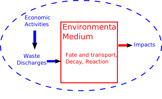
Conceptual Model of an Environmental System
  • Municipal sewage into lakes, rivers, etc.
  • Power plant emissions into air
  • Solid waste placed on landfill
  • CO2 into atmosphere

Other Aspects of Models

  • Deterministic vs. Stochastic
  • Descriptive vs. Prescriptive
  • Mechanistic vs. Statistical

“All Models Are Wrong, But Some Are Useful”

…all models are approximations. Essentially, all models are wrong, but some are useful. However, the approximate nature of the model must always be borne in mind….

— Box & Draper, Empirical Model Building and Response Surfaces, 1987

Questions?

Poll Everywhere QR Code

Text: VSRIKRISH to 22333

URL: https://pollev.com/vsrikrish

See Results

System Boundaries

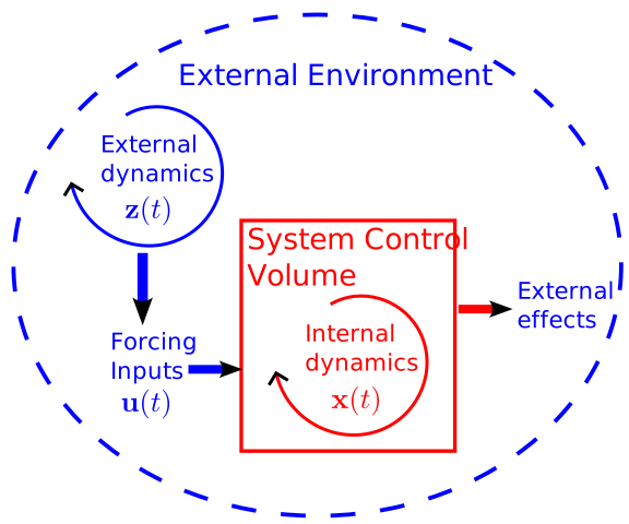
Defining the System Scope

  • “Internal” system dynamics vs. “external” conditions is somewhat arbitrary.
  • Internal dynamics go into a model.
  • External conditions are “forcings,” initial conditions, or assumptions.

Conceptual Model of an Environmental System

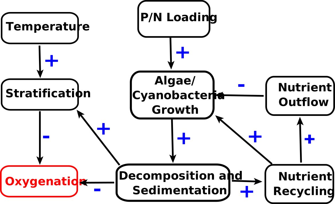
Example: Lake Eutrophication

Simple model of lake eutrophication:

Assume steady-state behavior, first-order linear decay, well-mixed, constant volume.

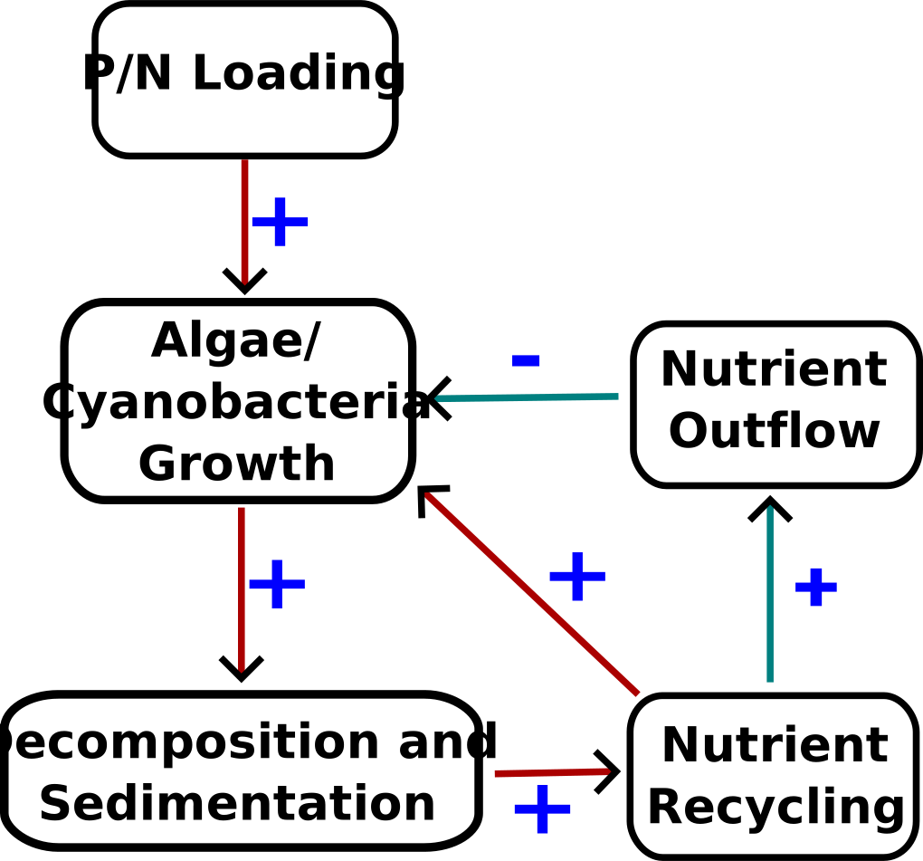
Adding more complexity:

Schematic of processes resulting in lake eutrophication

Systems Diagrams

Schematic of processes resulting in lake eutrophication

Example: EV Life Cycle Assessment

What factors contribute to the environmental impact of a battery electric vehicle (versus an internal combustion engine)?

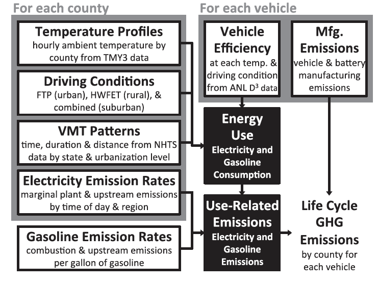
Possible System/Life Cycle Framework

Schematic of PHEV LCA Framework

::: {.caption}G Source: Yuksel et al. (2016) :::

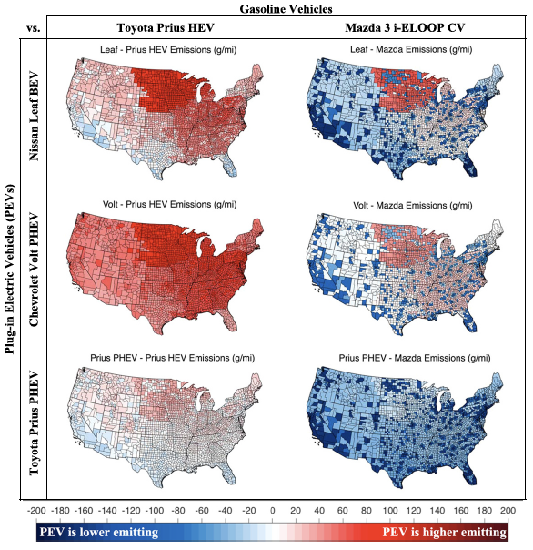
PHEV vs. Gasoline Outcomes

PHEV Comparison

Source: Yuksel et al. (2016)

Constructing Systems Models

Similar principles to models you’ve seen previously:

  • Mass/Energy Balance for stocks;
  • Flows can increase stocks or can decay.

Main difference: potential presence of feedbacks/non-steady state behavior.

Feedbacks

Feedback Types

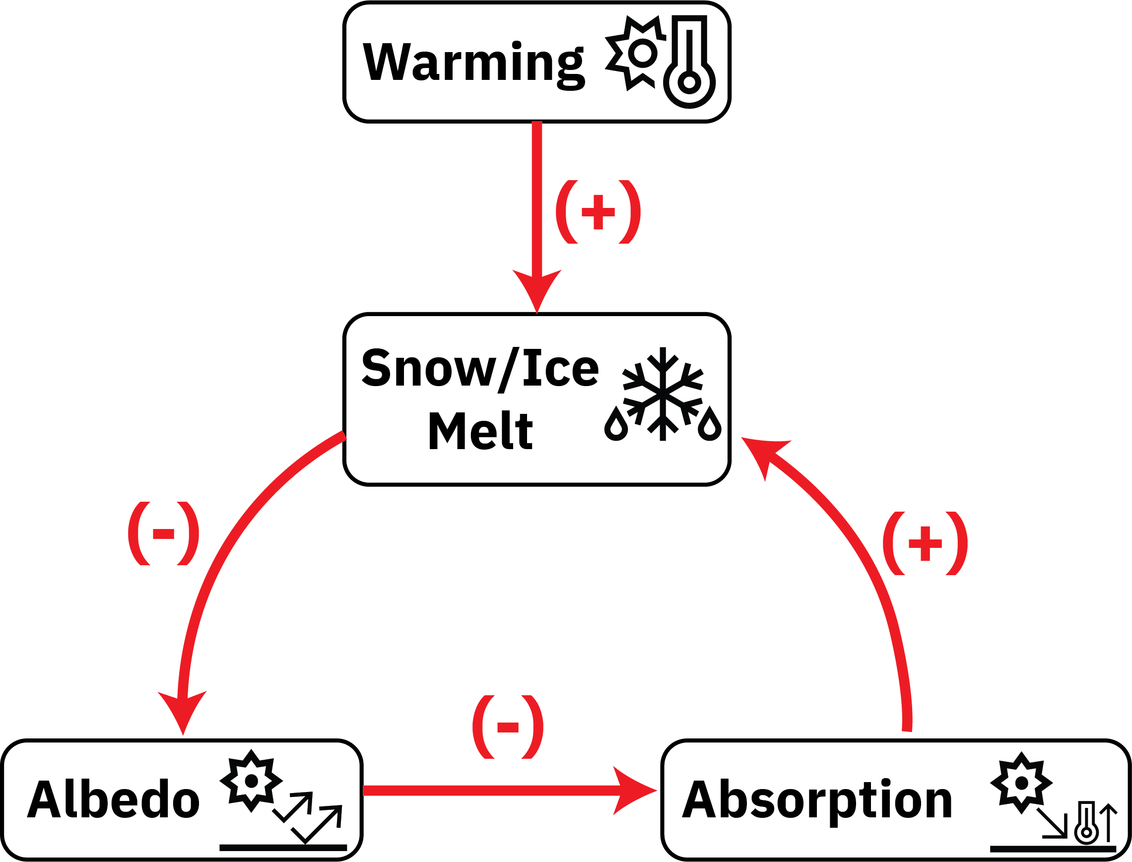
Feedbacks are “loops” in a system diagram.

Feedbacks can be:

  • Amplifying (sometimes called “positive”)
  • Dampening (sometimes called “negative”)

Ice-Albedo Feedback Loop

Amplifying Feedbacks

Shocks will amplify as they are propagated:

Amplifying Feedback Example

Dampening Feedbacks

Shocks are attenuated (dampened) as they propagate:

Dampening Feedback Example

Feedback Level

With no feedback: \(\text{Total Effect} = \text{Direct Effect}\)

Over one pass feedback loop: \(\text{Total Effect} = (1+g) (\text{Direct Effect})\)

\(g\) is the feedback factor (or gain): \(g > 0\) means amplification, \(g < 0\) means dampening.

Calculating \(g\)

If \(x = F[p(x, \ldots)]\), \[g = \frac{\partial F}{\partial x} = \frac{\partial F}{\partial p} \frac{\partial p}{\partial x}.\]

With multiple feedback processes (\(x = F[p_1(x, \ldots), p_2(x, \ldots), \ldots]\)):

\[g = \sum_i \frac{\partial F}{\partial p_i} \frac{\partial p_i}{\partial x} = \sum_i g_i.\]

Multiple Feedback Passes

\[\begin{aligned} \text{Total Effect} &= (\text{Direct Effect})\left(1 + g + g^2 + g^3 + \ldots\right) \\[0.5em] &= \frac{\text{Direct Effect}}{1-g} \end{aligned}\]

  • if \(0 < g < 1\): amplifying but stable feedback
  • if \(g < 0\): dampening feedback
  • if \(g > 1\): system instability

Other Environmental Feedbacks

Can we think of other examples of environmental feedback loops?

Are they amplifying or dampening?

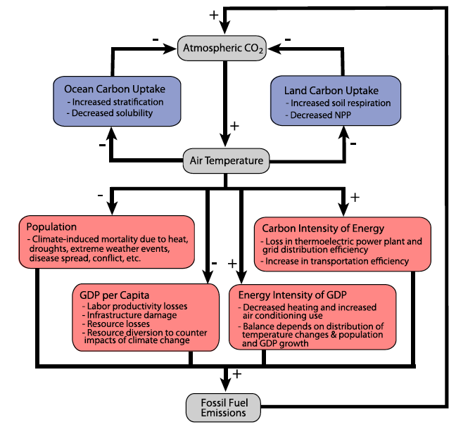
Example: Climate-Economic Feedbacks

Climate System Feedbacks

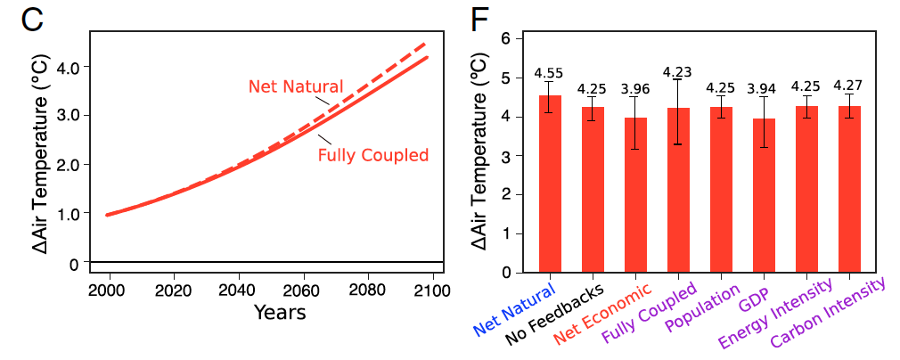
Climate Feedbacks Comparisons

Source: Woodard et al. (2019)

Impact of Including Feedbacks

Climate Feedbacks Comparisons

Source: Woodard et al. (2019)

Equilibria

Fixed Points (Equilibria)

System dynamics are often understood relative to their equilibria (or fixed points).

  • If \(X_{t+1} = F(X_t)\), equilibria occur where \(F(X_t) = X_t\).
  • If \(\frac{dx}{dt} = f(x)\), equilibria occur where \(f(x) = 0\).

In other words, a system at an equilibrium will stay at an equilibrium.

Example: Predator-Prey Dynamics

Code
lh_obs = DataFrame(CSV.File("data/lynx_hare/Lynx_Hare.txt", header=[:Year, :Hare, :Lynx]))[:, 1:3]
plot(lh_obs[!, :Year], lh_obs[!, :Lynx], xlabel="Year", ylabel="Pelts (thousands)", markersize=5, markershape=:circle, markercolor=:red, color=:red, linewidth=3, label="Lynx")
plot!(lh_obs[!, :Year], lh_obs[!, :Hare], markersize=5, markershape=:circle, markercolor=:blue, color=:blue, linewidth=3, label="Hare")
plot!(size=(1100, 500))
1860 1880 1900 1920 Year 0 50 100 150 Pelts (thousands) Lynx Hare
Figure 1: Lynx and Hare pelt dataset

Predator-Prey Dynamics (Lotka-Volterra)

\[ \begin{align*} \frac{dH}{dt} &= H_t \underbrace{b_H}_{\substack{\text{birth} \\ \text{rate}}} - H_t (\underbrace{L_t m_H}_{\substack{\text{impact of} \\ \text{lynxes}}}) \\ \frac{dL}{dt} &= L_t\underbrace{(H_t b_L)}_{\substack{\text{impact of} \\ \text{hares}}} - \underbrace{L_t m_L}_{\substack{\text{mortality} \\ \text{rate}}} \end{align*} \]

Lotka-Volterra Fixed Points

Code
function lotka_volterra!(du, u, p, t)
  # Unpack the values so that they have clearer meaning
  prey, pred  = u
  birth_prey, mort_prey, birth_pred, mort_pred = p

  # Define the ODE
  du[1] = (birth_prey - mort_prey * pred) * prey
  du[2] = (birth_pred * prey - mort_pred) * pred
end

# define model parameters and initial conditions
θ = [1.1, 0.5, 0.1, 0.2]
u₀ = [1, 1]
tspan = 40
prob = ODEProblem(lotka_volterra!, u₀, (0.0, tspan), θ)


# plot phase space
p = plot(xlims=(0, 10), ylims=(0, 6),
    xlabel = "Prey Population (1,000)", ylabel = "Predator Population (1,000)", leg = false)

function phase_plot(prob, u0, θ, p, tspan = 40)
    _prob = ODEProblem(prob.f, u0, tspan, θ)
    sol = solve(_prob, Vern9()) # Use Vern9 solver for higher accuracy
    plot!(p, sol, idxs = (1, 2))
end

for x in 0:0.5:2.5
    for y in 0:0.5:2.5
        phase_plot(prob, [y, x], θ, p)
    end
end

scatter!(p, [0, 2], [0, 2.2], color=:black)
plot!(size=(650, 550))
0 2 4 6 8 10 Prey Population (1,000) 0 1 2 3 4 5 6 Predator Population (1,000)
Figure 2: Phase Diagram of the Lotka-Volterra Equations

This simple model has two fixed points:

  1. \(L_t = 0, H_t = 0\)
  2. \(L_t = b_H / m_H, H_t = m_L / b_L\)

Paradox of the Pesticides

Improving the birth rate for the prey (increasing \(b_H\)) does not impact the equilibrium prey population, but benefits predators.

Killing more of the prey (increasing \(m_H\)) similarly impacts predators, not prey.

A similar impact was seen with pesticide deployment: led to widespread die-offs of natural predators of crop pest species, allowing increased flareups of pests.

Iron Fertilization

Another example: iron fertilization (increased phytoplankton are consumed by fish and other predators, decreasing observed carbon sequestration).

Key Takeaways

Key Takeaways

  • Definition of system boundary strongly influences modeled dynamics and assessments of outcome s (e.g. life-cycle assessment or attribution of effects);
  • Feedbacks can be amplifying or dampening;
  • Systems can include both types of feedbacks: overall effect depends on specifics!
  • Equilibria are “fixed points” of the system: more next time!

Upcoming Schedule

Next Classes

Wednesday: Stability and Bifurcations

Next Week: Labor Day (Monday); Quiz 1 (Wednesday)

Assessments

Homework 1: Due Thursday at 9pm.

References

References

Woodard, D. L., Davis, S. J., & Randerson, J. T. (2019). Economic carbon cycle feedbacks may offset additional warming from natural feedbacks. Proceedings of the National Academy of Sciences, 116, 759–764. https://doi.org/10.1073/pnas.1805187115
Yuksel, T., Tamayao, M.-A. M., Hendrickson, C., Azevedo, I. M. L., & Michalek, J. J. (2016). Effect of regional grid mix, driving patterns and climate on the comparative carbon footprint of gasoline and plug-in electric vehicles in the United States. Environ. Res. Lett., 11, 044007. https://doi.org/10.1088/1748-9326/11/4/044007